Chapter 3 Probability Distributions
3.1 Introduction
Combinatorial probabilities from the previous chapter are often problem-specific and tedious to compute. This chapter introduces structured approaches that make probability calculations easier. We represent outcomes of random experiments as values of a random variable, which lets us compute probabilities efficiently in many realistic, stylised settings.
3.2 Random variables
3.2.1 Introduction
This section introduces probability distributions of random variables via their probability functions. For discrete variables the probability function is the probability mass function (pmf); for continuous variables it is the probability density function (pdf).
A random variable maps each outcome in the sample space to a real number. For example, consider a fair coin toss with outcomes head or tail. Define the random variable that maps head to 1 and tail to 0: \[\text{Head} \rightarrow 1, \text{Tail} \rightarrow 0.\]
We can conveniently denote the random variable by \(X\) which is the number of heads obtained by tossing a single coin. The possible values of \(X\) are \(0\) and \(1\).
This is a simple example, and the idea generalises directly: define a function from outcomes to real numbers. For instance, toss a coin \(n\) times and let \(X\) be the number of heads; then \(X\) takes integer values from \(0\) to \(n\). As another example, select a student at random and measure their height. The resulting value, in metres, lies on a continuum (e.g., 1.432 m), and we cannot know it in advance because the selected student is random.
We use uppercase letters (e.g., \(X\), \(Y\), \(Z\)) for random variables and the corresponding lowercase letters (e.g., \(x\), \(y\), \(z\)) for particular values (e.g., \(x=1.432\) m). We also write probabilities as \(P(X \in A)\), read “the probability that \(X\) lies in \(A\),” instead of \(P\{A\}\).
3.2.2 Discrete and continuous random variables
A random variable is discrete if it takes a finite or countably infinite set of values (e.g., the number of Apple users among 20 students; the number of credit cards a person carries). It is continuous if it can take any real value (e.g., a student’s height). Some variables mix discrete and continuous parts (e.g., daily rainfall: zero on some days, a positive continuous amount on others).
3.2.3 Probability distribution of a random variable
By the first axiom of probability, total probability is 1. Because a random variable maps outcomes to the real line, the probabilities assigned to all its possible values must sum (or integrate) to 1. A probability distribution allocates this total probability across those values.
Example 3.1 Returning to the coin-tossing experiment, if the probability of getting a head with a coin is \(p\) (and therefore the probability of getting a tail is \(1 - p\)), then the probability that \(Y = 0\) is \(1 - p\) and the probability that \(Y = 1\) is \(p\). This gives us the probability distribution of \(Y\), and we say that \(Y\) has the probability function \[P(Y = y) = \begin{cases} 1-p & \text{for $y = 0$} \\ p & \text{for $y = 1$.} \end{cases}\] This is an example of the Bernoulli distribution with parameter \(p\), the simplest discrete distribution.
Example 3.2 Suppose we consider tossing the coin twice and again defining the random variable \(X\) to be the number of heads obtained. The values that \(X\) can take are \(0\), \(1\) and \(2\) with probabilities \((1 - p)^2\) , \(2p(1 - p)\) and \(p^2\), respectively. Here the probability function is \[P(X = x) = \begin{cases} (1 - p)^2 & \text{for $x = 0$} \\ 2p(1 - p) & \text{for $x = 1$} \\ p^2 & \text{for $x = 2$.} \end{cases}\] This is a particular case of the Binomial distribution. We will learn about it soon.
In general, for a discrete random variable we define a function \(f(x)\) to denote \(P (X = x)\) (or \(f (y)\) to denote \(P (Y = y)\)) and call the function \(f (x)\) the probability mass function (pmf) of \(X\). Not every function qualifies: probabilities are nonnegative and sum to 1. Thus, for \(f(x)\) to be a pmf of \(X\), we require:
- \(f (x) \geq 0\) for all possible values of \(x\).
- \(\sum_{\text{all $x$}} f (x) = 1\)
In Example 3.2, we may rewrite the probability function in the general form \[f(x) = \binom{2}{x} p^x (1 - p)^{2-x}, \text{for $x = 0, 1, 2$},\] where \(f (x) = 0\) for any other value of \(x\).
3.2.4 Continuous random variables
In many situations (both theoretical and practical) we often encounter random variables that are inherently continuous because they are measured on a continuum (such as time, length, weight) or can be conveniently well-approximated by considering them as continuous (such as the annual income of adults in a population, closing share prices).
For a continuous random variable, \(P(X=x)=0\) for any specific \(x\) (e.g., exactly 1.2), because measurements lie on a continuum. Instead, we assign probabilities to intervals with positive length, such as \(P(1.2<X<1.9)\).
For a continuous random variable \(X\), probabilities derive from a nonnegative function \(f(x)\), the probability density function (pdf). We compute probabilities via integrals, e.g., \[P (a < X < b) = \int_a^b f (u) du,\] which is naturally interpreted as the area under the curve \(f (x)\) inside the interval \((a, b)\). This is demonstrated in Figure 3.1. Recall that we do not use \(f (x) = P (X = x)\) for any \(x\) as by convention we set \(P(X = x) = 0\).
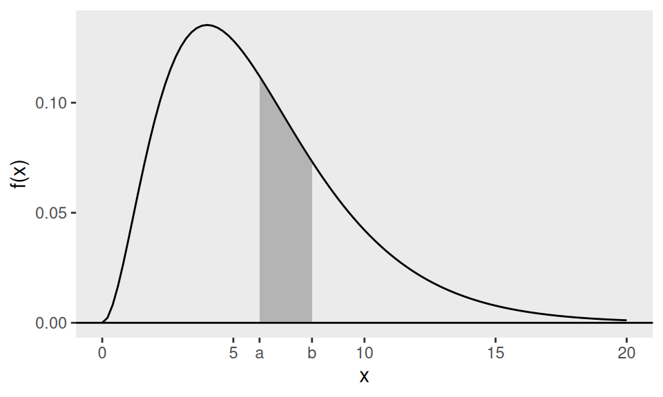
Figure 3.1: The shaded area is \(P (a < X < b)\) if the pdf of \(X\) is the drawn curve.
Since we are dealing with probabilities which are always between \(0\) and \(1\), just any arbitrary function f (x) cannot be a pdf of some random variable. For \(f (x)\) to be a pdf, as in the discrete case, we must have
- \(f (x) \geq 0\) for all possible values of \(x\), i.e. \(-\infty < x < \infty\),
- \(\int_{-\infty}^{\infty} f (u)du = 1\).
3.2.5 Cumulative distribution function (cdf)
We also use the cumulative distribution function (cdf), which gives the probability that the random variable is less than or equal to a given value.
For a discrete random variable \(X\), the cdf is the cumulative sum of the pmf \(f(u)\) up to (and including) \(u = x\). That is, \[P (X \leq x) \equiv F (x) = \sum_{u \leq x} f (u).\]
Example 3.3 Let \(X\) be the number of heads in the experiment of tossing two fair coins. Then the probability function is \[P (X = 0) = 1/4, \; P (X = 1) = 1/2, \; P (X = 2) = 1/4.\]
From the definition, the CDF is given by \[F(x)= \begin{cases}0 & \text { if } x<0 \\ 1 / 4 & \text { if } 0 \leq x<1 \\ 3 / 4 & \text { if } 1 \leq x<2 \\ 1 & \text { if } x \geq 2\end{cases}\]
The cdf for a discrete random variable is a step function. The jump-points are the possible values of the random variable, and the height of a jump gives the probability of the random variable taking that value. It is clear that the probability mass function is uniquely determined by the cdf.
For a continuous random variable \(X\), the cdf is defined as \[P (X \leq x) \equiv F (x) = \int_{-\infty}^x f (u)du.\]
The fundamental theorem of calculus then tells us that \[f (x) = \frac{dF (x)}{dx},\] so for a continuous random variable the pdf is the derivative of the cdf. Also for any random variable \(X\), \(P (c < X \leq d) = F (d) - F (c)\). Let us consider an example.
Example 3.4 (Uniform distribution) Suppose \[f(x)= \begin{cases}\frac{1}{b-a} & \text { if } a<x<b \\ 0 & \text { otherwise.}\end{cases}\] In this case we say X has uniform distribution on the interval \((a, b)\), which we will write as \(X \sim U(a, b)\). We now have the cdf \[F(x)=\int_{a}^{x} \frac{1}{b-a} du =\frac{x-a}{b-a}, \; \; a<x<b.\] A quick check confirms that \(F^{\prime}(x)=f(x)\). If \(a=0\) and \(b=1\), then \[P(0.5<X<0.75)=F(0.75)-F(0.5)=0.25.\] We will see more examples later.
3.3 Summaries of a random variable
3.3.1 Introduction
In Section 1.4, we defined various summaries of sample data \(x_1 , \ldots , x_n\), such as the mean and variance. A random variable \(X\) with either a pmf \(f (x)\) or a pdf \(f (x)\) may be summarised using similar measures.
3.3.2 Expectation
The mean of \(X\), or expectation, is defined as \[E(X)= \begin{cases}\sum_{\text{all $x$}} x f(x) & \text { if } X \text { is discrete } \\ \int_{-\infty}^{\infty} x f(x) d x & \text { if } X \text { is continuous }\end{cases}\] when the sum or integral exists. Informally, expectation is the sum or integral of “value × probability.” We write \(E(\cdot)\) for expectation and often denote \(E(X)\) by \(\mu\).
Example 3.5 Consider the fair-die tossing experiment, with each of the six sides having a probability of \(1 / 6\) of landing face up. Let \(X\) be the number on the up-face of the die. Then \[E(X)=\sum_{x=1}^{6} x P(X=x)=\sum_{x=1}^{6} x / 6=3.5.\]
Example 3.6 Suppose \(X \sim U(a, b)\), with pdf \(f(x)=\frac{1}{b-a}, \, a<x<b.\) Then \[\begin{align*} E(X) &=\int_{-\infty}^{\infty} x f(x) d x \\ &=\int_{a}^{b} \frac{x}{b-a} d x \\ &=\frac{b^{2}-a^{2}}{2(b-a)}=\frac{b+a}{2}, \end{align*}\] the mid-point of the interval \((a, b)\).
If \(Y=g(X)\) for any function \(g(\cdot)\), then \(Y\) is a random variable as well. To find \(E(Y)\) we simply use the value times probability rule, i.e. the expected value of \(Y\) is either sum or integral of its value, \(g(x)\), times probability \(f(x)\): \[E(Y)=E(g(X))=\begin{cases} \sum_{\text{all $x$}} g(x) f(x) & \text { if $X$ is discrete, } \\ \int_{-\infty}^{\infty} g(x) f(x) d x & \text { if $X$ is continuous.} \end{cases}\]
For example, if \(X\) is continuous, then \(E(X^2) = \int_{-\infty}^{\infty} x^2 f(x) dx\). We prove an important property of expectation, namely expectation is a linear operator.
Theorem 3.1 (Linearity of expectation) If \(Y=aX+b\), then \(E(Y)=a\,E(X)+b\).
Proof. The proof is given for the continuous case. In the discrete case replace integral (\(\int\)) by summation (\(\sum\)). \[\begin{align*} E(Y ) &= \int_{-\infty}^\infty (ax + b) f(x)dx \\ &= a \int_{-\infty}^\infty x f (x)dx + b \int_{-\infty}^\infty f (x)dx \\ &= aE(X) + b, \end{align*}\] using the total probability is 1 property (\(\int_{-\infty}^\infty f (x)dx = 1\)) in the last integral.
This is very convenient, e.g. suppose \(E(X) = 5\) and \(Y = -2X + 549\) then \(E(Y) = 539\).
We will also prove an important property of expectation for symmetric random variables.
Theorem 3.2 If the pmf/pdf of \(X\) is symmetric about \(c\) (i.e., \(f(c+x)=f(c-x)\) for all \(x>0\)), then \(E(X)=c\).
Proof. The proof is given for the continuous case. In the discrete case replace integral (\(\int\)) by summation (\(\sum\)).
First, let \(Y = X - c\). Then \(Y\) is symmetric about \(0\), with probability density function \(f(y) = f(-y)\) for all \(y >0\). Then \[\begin{align*} E(Y) &= \int_{-\infty}^\infty y f(y) dy \\ &= \int_{-\infty}^0 y f(y) dy + \int_0^\infty y f(y) dy \\ &= \int_{0}^\infty -z f(-z) dz + \int_0^\infty y f(y) dy, \text{ substituting $z = -y$} \\ &= - \int_{0}^\infty z f(z) dz + \int_0^\infty y f(y) dy, \text{ since $f(-z) = f(z)$} \\ &= 0. \end{align*}\] So, by the linearity of expectation, \(E(X) = E(Y + c) = E(Y) + c = 0 + c = c.\)
This result makes it very easy to find the expectation of any symmetric random variable. The two examples we saw before, of a fair die and of a uniform random variable, were both symmetric, and they have expectation equal to the point of symmetry.
3.3.3 Variance
Variance measures the spread of a random variable and is defined by \[\operatorname{Var}(X)=E(X-\mu)^{2}= \begin{cases} \sum_{\text {all } x}(x-\mu)^{2} f(x) & \text { if $X$ is discrete} \\ \int_{-\infty}^{\infty}(x-\mu)^{2} f(x) dx & \text { if $X$ is continuous,} \end{cases}\] where \(\mu=E(X)\), and when the sum or integral exists. When the variance exists, it is the expectation of \((X-\mu)^{2}\) where \(\mu\) is the mean of \(X\). A useful identity is:
Theorem 3.3 \[\operatorname{Var}(X)=E(X-\mu)^{2}=E\left(X^{2}\right)-\mu^{2}.\]
Proof. We have \[\begin{align*} \operatorname{Var}(X) &=E(X-\mu)^{2} \\ &=E\left(X^{2}-2 X \mu+\mu^{2}\right) \\ &=E\left(X^{2}\right)-2 \mu E(X)+\mu^{2} \\ &=E\left(X^{2}\right)-2 \mu \mu+\mu^{2} \\ &=E\left(X^{2}\right)-\mu^{2}. \end{align*}\]
Thus, variance equals the expected square minus the square of the mean. We denote variance by \(\sigma^2\), which is always nonnegative and equals zero only if \(X=\mu\) with probability 1 (no randomness). The square root, \(\sigma\), is the standard deviation.
Example 3.7 (Uniform distribution) Suppose \(X \sim U(a, b)\), with pdf \(f(x)=\frac{1}{b-a}, \, a<x<b.\) Then \[\begin{align*} E\left(X^{2}\right) &=\int_{a}^{b} \frac{x^{2}}{b-a} d x \\ &=\frac{b^{3}-a^{3}}{3(b-a)} \\ &=\frac{b^{2}+a b+a^{2}}{3}. \end{align*}\] Hence \[\operatorname{Var}(X)=\frac{b^{2}+a b+a^{2}}{3}-\left(\frac{b+a}{2}\right)^{2}=\frac{(b-a)^{2}}{12},\] after simplification.
We prove one important property of the variance.
Theorem 3.4 Suppose \(Y=a X+b\) then \(\operatorname{Var}(Y)=a^{2} \operatorname{Var}(X)\)
Proof. Write \(\mu = E(X)\). Then \(E(Y) = a\mu + b\) and \[\begin{align*} \operatorname{Var}(Y) &=E\left[(Y-E(Y))^{2}\right] \\ &=E\left[(aX + b - a\mu - b)^2\right] \\ &=E\left[a^2(X -\mu)^2\right] \\ &=a^2 E\left[(X -\mu)^2\right] \\ &=a^{2} \operatorname{Var}(X) \end{align*}\]
This is a very useful result, e.g. suppose \(\operatorname{Var}(X)=25\) and \(Y=-X+5,000,000\); then \(\operatorname{Var}(Y)=\) \(\operatorname{Var}(X)=25\) and the standard deviation, \(\sigma=5\). In words a location shift, \(b\), does not change variance but a multiplicative constant, \(a\) say, gets squared in variance, \(a^{2}\).
3.3.4 Quantiles
For \(0<p<1\), a \(p\)th quantile (or \(100p\)th percentile) of \(X\) with cdf \(F\) is any \(q\) such that \(F(q)=p\). If \(F\) is invertible, \(q=F^{-1}(p)\).
The 50th percentile is called the median. The 25th and 75th percentiles are called the quartiles.
Example 3.8 (Uniform distribution) Suppose \(X \sim U(a, b)\), with pdf \(f(x)=\frac{1}{b-a}, \, a<x<b.\) We have shown in Example 3.4 that the cdf is \[F(x)=\frac{x-a}{b-a}, \; a<x<b.\] So for a given \(p\), \(F(q)=p\) implies \[q=a+p(b-a).\] The median of \(X\) is \(\frac{b+a}{2}\) and the quartiles are \(\frac{b + 3a}{4}\) and \(\frac{3b + a}{4}\).
The median of a symmetric random variable is the point of symmetry: ::: {.theorem} Suppose \(X\) is a random variable with a probability function or probability density function which is symmetric about some value \(c\), so \[f(c + x) = f(c - x) \text{ for all $x >0$.}\] Then the median of \(X\) is \(c\). :::
3.4 Standard discrete distributions
3.4.1 Bernoulli distribution
Bernoulli trials are independent trials with two outcomes (success S, failure F) and common success probability.
Suppose that we conduct one Bernoulli trial, where we get a success \((S)\) or failure \((F)\) with probabilities \(P\{S\}=p\) and \(P\{F\}=1-p\) respectively. Let \(X\) be an indicator of success: \[X = \begin{cases} 1 & \text{if $S$} \\ 0 & \text{if $F$.} \end{cases}\] Then \(X\) has Bernoulli distribution with parameter \(p\), written as \(X \sim \operatorname{Bernoulli}(p)\).
The Bernoulli distribution has pmf \[f(x)=p^{x}(1-p)^{1-x}, x=0,1.\] Hence \[E(X)=0 \cdot(1-p)+1 \cdot p=p,\] \[E\left(X^{2}\right)=0^{2} \cdot(1-p)+1^{2} \cdot p=p\] and \[\operatorname{Var}(X)=E\left(X^{2}\right)-(E(X))^{2}=p-p^{2}=p(1-p).\]
3.4.2 Binomial distribution
3.4.2.1 Introduction and definition
In \(n\) independent Bernoulli trials with success probability \(p\), let \(X\) be the number of successes. Then \(X \sim \operatorname{Bin}(n,p)\) with \(X \sim \operatorname{Bin}(n, p)\).
An outcome of the experiment (of carrying out \(n\) such independent trials) is represented by a sequence of \(S\)’s and \(F\)’s (such as \(S S \ldots F S \ldots S F)\) that comprises \(x\) \(S\) ’s, and \((n-x)\) \(F\) ’s. The probability associated with this outcome is \[P\{S S \ldots F S \ldots S F\}=p p \cdots(1-p) p \cdots p(1-p)=p^{x}(1-p)^{n-x}.\] For this sequence, \(X=x\), but there are many other sequences which will also give \(X=x\). In fact there are \(\binom{n}{x}\) such sequences. Hence \[P(X=x)= \binom{n}{x} p^{x}(1-p)^{n-x}, x=0,1, \ldots, n .\] This is the pmf of the binomial distribution with parameters \(n\) and \(p\)
How can we guarantee that \(\sum_{x=0}^{n} P(X=x)=1\)? This guarantee is provided by the binomial theorem:
Theorem 3.5 (Binomial theorem) For any positive integer \(n\) and real numbers \(a\) and \(b\), \[(a+b)^{n}=b^{n}+ \binom{n}{1} a b^{n-1}+\cdots+\binom{n}{x} a^x b^{n-x}+\cdots +a^{n}.\]
Setting \(a=p\) and \(b=1-p\) in the binomial theorem shows \(\sum_{x=0}^{n}\binom{n}{x} p^{x}(1-p)^{n-x}=1\).
Example 3.9 Suppose that widgets are manufactured in a mass production process with \(1\%\) defective. The widgets are packaged in bags of 10 with a money-back guarantee if more than 1 widget per bag is defective. For what proportion of bags would the company have to provide a refund?
First, we find the probability that a randomly selected bag has at most 1 defective widget. Let \(X\) be the number of defective widgets in a bag, then \(X \sim \operatorname{Bin}(n = 10, p = 0.01).\) So this probability is equal to \[P (X = 0) + P (X = 1) = (0.99)^{10} + 10(0.01)^1 (0.99)^9 = 0.9957.\] Hence the probability that a refund is required is \(1 - 0.9957 = 0.0043\), i.e. only just over 4 in 1000 bags will incur the refund on average.
Example 3.10 A binomial random variable can also be described using the urn model. Suppose we have an urn (population) containing \(N\) individuals, a proportion \(p\) of which are of type \(S\) and a proportion \(1 - p\) of type \(F\). If we select a sample of \(n\) individuals at random with replacement, then the number, \(X\), of type \(S\) individuals in the sample follows the binomial distribution with parameters \(n\) and \(p\).
3.4.2.2 Using R to calculate probabilities
Probabilities under all the standard distributions have been calculated in R and will be used throughout MATH1063. You will not be required to use any tables. For the binomial distribution the command
calculates the pmf of \(\operatorname{Bin}(n = 5, p = 0.34)\) at \(x=3\),
with value \(P (X = 3) = \binom{5}{3} (0.34)^3 (1 - 0.34)^{5-3}\).
The function pbinom returns the cdf (probability up to and including the argument). Thus
will return the value of \(P (X \leq 3)\) when \(X \sim \operatorname{Bin}(n = 5, p = 0.34)\). As a check, in Example 3.9, we may compute the probability that a randomly selected bag has at most 1 defective widget with the command
## [1] 0.9957338which matches our earlier calculations.
3.4.2.3 Expectation
Let \(X \sim \operatorname{Bin}(n, p)\). We have \[E(X)=\sum_{x=0}^{n} x P(X=x)=\sum_{x=0}^{n} x \binom{n}{x} p^{x}(1-p)^{n-x}.\] Below we prove that \(E(X)=n p\). Recall that \(k !=k(k-1) !\) for any \(k>0\). \[\begin{align*} E(X) &=\sum_{x=0}^{n} x \binom{n}{x} p^{x}(1-p)^{n-x} \\ &=\sum_{x=1}^{n} x \frac{n!}{x !(n-x)!} p^{x}(1-p)^{n-x} \\ &=\sum_{x=1}^{n} \frac{n !}{(x-1) !(n-x) !} p^{x}(1-p)^{n-x} \\ &=n p \sum_{x=1}^{n} \frac{(n-1) !}{(x-1) !(n-1-x+1) !} p^{x-1}(1-p)^{n-1-x+1} \\ &=n p \sum_{y=0}^{n-1} \frac{(n-1) !}{y!(n-1-y)!} p^{y}(1-p)^{n-1-y} \\ &=n p \sum_{y=0}^{n-1} \binom{n-1}{y} p^{y}(1-p)^{n-1-y} \\ &=n p \end{align*}\] where we used the substitution \(y=x-1\) and then conclude the last sum equals one as it is the sum of all probabilities in the \(\operatorname{Bin}(n-1, p)\) distribution.
3.4.2.4 Variance
Let \(X \sim \operatorname{Bin}(n, p)\). Then \(\operatorname{Var}(X)=n p(1-p)\). It is difficult to find \(E\left(X^{2}\right)\) directly, but the factorial structure allows us to find \(E[X(X-1)]\). Recall that \(k !=k(k-1)(k-2) !\) for any \(k>1\). \[\begin{align*} E[(X(X-1)]&=\sum_{x=0}^{n} x(x-1) \binom{n}{x} p^{x}(1-p)^{n-x} \\ &=\sum_{x=2}^{n} x(x-1) \frac{n !}{x !(n-x) !} p^{x}(1-p)^{n-x} \\ &=\sum_{x=2}^{n} \frac{n !}{(x-2) !(n-x) !} p^{x}(1-p)^{n-x} \\ &=n(n-1) p^{2} \sum_{x=2}^{n} \frac{(n-2) !}{(x-2) !(n-2-x+2) !} p^{x-2}(1-p)^{n-2-x+2} \\ &=n(n-1) p^{2} \sum_{y=0}^{n-2} \frac{(n-2) !}{(y) !(n-2-y) !} p^{y}(1-p)^{n-2-y} \\ &=n(n-1) p^2 \end{align*}\] where we used the substitution \(y=x-2\) and then conclude the last sum equals one as it is the sum of all probabilities in the \(\operatorname{Bin}(n-2, p)\) distribution. Now, \(E\left(X^{2}\right)=E[X(X-1)]+E(X)=n(n-1) p^{2}+n p\). Hence, \[\operatorname{Var}(X)=E\left(X^{2}\right)-(E(X))^{2}=n(n-1) p^{2}+n p-(n p)^{2}=n p(1-p).\] It is illuminating to see these direct proofs. Later on we shall apply statistical theory to directly prove these.
3.4.3 Geometric distribution
3.4.3.1 Introduction and definition
Suppose that we have the same situation as for the binomial distribution but we consider a different random variable \(X\), which is defined as the number of trials that lead to the first success. The outcomes for this experiment are: \[\begin{array}{rll} S & X=1, & P(X=1)=p \\ F S & X=2, & P(X=2)=(1-p) p \\ F F S & X=3, & P(X=3)=(1-p)^{2} p \\ F F F S & X=4, & P(X=4)=(1-p)^{3} p \\ \vdots & \vdots & \end{array}\] In general, \[P(X=x)=(1-p)^{x-1} p, \; x=1,2,\ldots\] This is the geometric distribution, supported on \(\{1,2,\ldots\}\), written \(X \sim \operatorname{Geo}(p)\).
Example 3.11 In a board game that uses a single fair die, a player cannot start until they have rolled a six. Let \(X\) be the number of rolls needed until they get a six. Then \(X\) is a Geometric random variable with success probability \(p = 1/6\).
In order to check the probability function sums to one, we will need to use the general result on the geometric series:
Theorem 3.6 (Geometric series) For any real numbers \(a\) and \(r\) such that \(|r| < 1\), \[\sum_{k=0}^\infty a r^k = \frac{a}{1-r}.\]
We now check the probability function sums to one: \[\begin{align*} \sum_{x=1}^{\infty} P(X=x) &=\sum_{x=1}^{\infty}(1-p)^{x-1} p \\ &=\sum_{y=0}^{\infty}(1-p)^{y} p \quad \text{(substitute $y=x-1$)} \\ &= \frac{p}{1-(1-p)} \quad \text{(geometric series, $a=p$, $r=1-p$)} \\ &=1 \end{align*}\] We can also find the probability that \(X>k\) for some given positive integer \(k\) : \[\begin{align*} \sum_{x=k+1}^{\infty} P(X=x) &=\sum_{x=k+1}^{\infty}(1-p)^{x-1} p \\ &=p\left[(1-p)^{k+1-1}+(1-p)^{k+2-1}+(1-p)^{k+3-1}+\ldots\right]\\ &=p(1-p)^{k} \sum_{y=0}^{\infty}(1-p)^{y} \\ &=(1-p)^{k} \end{align*}\]
3.4.3.2 Memoryless property
Let \(X\) follow the geometric distribution and suppose that \(s\) and \(k\) are positive integers. We then have \[P(X>s+k \mid X>k)=P(X>s).\]
This means the process “forgets” how long it has already waited: the remaining wait distribution is the same as at time zero. Using the definition of conditional probability, \[P\{A \mid B\}=\frac{P\{A \cap B\}}{P\{B\}}.\] Now the proof, \[\begin{align*} P(X>s+k \mid X>k) &=\frac{P(X>s+k, X>k)}{P(X>k)} \\ &=\frac{P(X>s+k)}{P(X>k)} \\ &=\frac{(1-p)^{s+k}}{(1-p)^{k}} \\ &=(1-p)^{s}, \end{align*}\] which does not depend on \(k\). Note that the event \(X>s+k\) and \(X>k\) implies and is implied by \(X>s+k\) since \(s>0\).
3.4.3.3 Expectation and variance
Let \(X \sim \operatorname{Geo}(p)\). We can show that \(E(X)=1/p\) using the negative binomial series:
Theorem 3.7 (Negative binomial series) For any positive integer \(n\) and real number \(x\) such that \(|x|<1\) \[(1-x)^{-n}=1+n x+\frac{1}{2} n(n+1) x^{2}+\frac{1}{6} n(n+1)(n+2) x^{3}+\cdots+\frac{n(n+1)(n+2) \cdots(n+k-1)}{k !} x^{k}+\cdots\]
We have \[\begin{align*} E(X) &=\sum_{x=1}^{\infty} x P(X=x) \\ &=\sum_{x=1}^{\infty} x p(1-p)^{x-1} \\ &=p\left[1+2(1-p)+3(1-p)^{2}+4(1-p)^{3}+\ldots\right] \end{align*}\] The series in the square brackets is the negative binomial series with \(n=2\) and \(x=1-p\). Thus \(E(X)=p(1-1+p)^{-2}=1 / p\). It can be shown that \(\operatorname{Var}(X)=(1-p) / p^{2}\) using negative binomial series. But this is more complicated and is not required here. The second-year module Statistical Inference will provide an alternative proof.
3.4.4 Hypergeometric distribution
Consider an urn with \(N\) individuals, of which a proportion \(p\) are type \(S\) and \(1-p\) are type \(F\). Sampling \(n\) without replacement, let \(X\) be the number of type \(S\); then \(X\) has the hypergeometric distribution, with pmf \[P(X=x)=\frac{\binom{Np}{x} \binom{N(1-p)}{n-x}}{\binom{N}{n}}, \quad x=0,1, \ldots, n,\] assuming that \(x \leq N p\) and \(n-x \leq N(1-p)\) so that the above combinations are well defined. The mean and variance of the hypergeometric distribution are given by \[E(X)=n p, \quad \operatorname{Var}(X)=n p (1-p) \frac{N-n}{N-1}.\]
3.4.5 Negative binomial distribution
In Bernoulli trials, let \(X\) be the total number of trials needed to observe the \(r\)th success, for a fixed positive integer \(r\). Then \(X\) follows the negative binomial distribution with parameters \(r\) and \(p\). [Note: if \(r = 1\), the negative binomial distribution is just the geometric distribution.] Firstly we need to identify the possible values of \(X\). Possible values for \(X\) are \(x = r, r + 1, r + 2, \ldots\). The probability mass function is \[\begin{align*} P (X = x) &= \binom{x-1}{r-1} p^{r-1} (1 - p)^{(x-1)-(r-1)} \times p \\ &=\binom{x-1}{r-1} p^r (1 - p)^{x-r}, \quad x = r, r + 1, \ldots \end{align*}\]
Example 3.12 A man plays roulette, betting on red each time. He decides to keep playing until he achieves his second win. The success probability for each game is \(18/37\) and the results of games are independent. Let \(X\) be the number of games played until he gets his second win. Then \(X\) is a negative binomial random variable with \(r = 2\) and p = \(18/37\).
What is the probability he plays more than \(3\) games? We have \[P (X > 3) = 1 - P(X = 2) - P(X = 3) = 1 - p^2 - 2 p^2 (1-p) = 0.520.\]
Derivation of the mean and variance of the negative binomial distribution involves complicated negative binomial series and will be skipped for now, but will be proved in Section \(\ref{sec:sum-rvs}\). For completeness we note down the mean and variance: \[E(X) = \frac{r}{p}, \quad \operatorname{Var}(X) = r \, \frac{1-p}{p^2}.\] Thus when r = 1, the mean and variance of the negative binomial distribution are equal to those of the geometric distribution.
3.4.6 Poisson distribution
3.4.6.1 Introduction and definition
The Poisson distribution arises as a limit of \(\operatorname{Bin}(n,p)\) when \(n \to \infty\), \(p \to 0\), and \(\lambda = np\) stays finite. It models counts of rare events. Its support is \(\{0,1,2,\ldots\}\). Examples include the number of cases in a region, the number of texts a student sends per day, or the number of credit cards a person carries.
Let us find the pmf of the Poisson distribution as the limit of the pmf of the binomial distribution. Recall that if \(X \sim \operatorname{Bin}(n, p)\) then \(P(X=x)=\left(\begin{array}{l}n \\ x\end{array}\right) p^{x}(1-p)^{n-x}\). Now: \[\begin{align*} P(X=x) &=\binom{n}{x} p^{x}(1-p)^{n-x} \\ &=\binom{n}{x} \frac{n^{n}}{n^{n}} p^{x}(1-p)^{n-x} \\ &=\frac{n(n-1) \cdots(n-x+1)}{n^{x} x !}(n p)^{x}(n(1-p))^{n-x} \frac{1}{n^{n-x}} \\ &=\frac{n}{n} \frac{(n-1)}{n} \cdots \frac{(n-x+1)}{n} \frac{\lambda^{x}}{x !}\left(1-\frac{\lambda}{n}\right)^{n-x}\\ &=\frac{n}{n} \frac{(n-1)}{n} \cdots \frac{(n-x+1)}{n} \frac{\lambda^{x}}{x !}\left(1-\frac{\lambda}{n}\right)^{n}\left(1-\frac{\lambda}{n}\right)^{-x}. \end{align*}\] Now it is easy to see that the above tends to \[e^{-\lambda} \frac{\lambda^{x}}{x!}\] as \(n \rightarrow \infty\) for any fixed value of \(x\) in the range \(0,1,2, \ldots .\) Note that we have used the exponential limit: \[e^{-\lambda}=\lim _{n \rightarrow \infty}\left(1-\frac{\lambda}{n}\right)^{n},\] and \[ \lim _{n \rightarrow \infty}\left(1-\frac{\lambda}{n}\right)^{-x}=1\] and \[ \lim _{n \rightarrow \infty} \frac{n}{n} \frac{(n-1)}{n} \cdots \frac{(n-x+1)}{n}=1.\] A random variable \(X\) has the Poisson distribution with parameter \(\lambda\) if it has the pmf: \[P(X=x)=e^{-\lambda} \frac{\lambda^{x}}{x !}, \quad x=0,1,2, \ldots\] We write \(X \sim \operatorname{Poisson}(\lambda)\). It is easy to show \(\sum_{x=0}^{\infty} P(X=x)=1\), i.e. \(\sum_{x=0}^{\infty} e^{-\lambda} \frac{\lambda^{x}}{x !}=1\). The identity you need is simply the expansion of \(e^{\lambda}\).
3.4.6.2 Expectation
Let \(X \sim \operatorname{Poisson}(\lambda)\). Then \[\begin{align*} E(X) &=\sum_{x=0}^{\infty} x P(X=x) \\ &=\sum_{x=0}^{\infty} x e^{-\lambda} \frac{\lambda^{x}}{x!} \\ &=e^{-\lambda} \sum_{x=1}^{\infty} x \frac{\lambda^{x}}{x !} \\ &=e^{-\lambda} \sum_{x=1}^{\infty} \frac{\lambda \cdot \lambda^{(x-1)}}{(x-1) !} \\ &=\lambda e^{-\lambda} \sum_{x=1}^{\infty} \frac{\lambda^{(x-1)}}{(x-1) !} \\ &=\lambda e^{-\lambda} \sum_{y=0}^{\infty} \frac{\lambda^{y}}{y !} \quad (y=x-1) \\ &=\lambda e^{-\lambda} e^{\lambda} \quad \text {using the expansion of $e^{\lambda}$} \\ &=\lambda . \end{align*}\]
3.4.6.3 Variance
Let \(X \sim \operatorname{Poisson}(\lambda)\). Then \[\begin{align*} E[X(X-1)] &=\sum_{x=0}^{\infty} x(x-1) P(X=x) \\ &=\sum_{x=0}^{\infty} x(x-1) e^{-\lambda} \frac{\lambda^{x}}{x!} \\ &=e^{-\lambda} \sum_{x=2}^{\infty} x(x-1) \frac{\lambda^{x}}{x !} \\ &=e^{-\lambda} \sum_{x=2}^{\infty} \lambda^{2} \frac{\lambda^{x-2}}{(x-2) !} \\ &=\lambda^{2} e^{-\lambda} \sum_{y=0}^{\infty} \frac{\lambda^{y}}{y !} \quad (y=x-2) \\ &=\lambda^{2} e^{-\lambda} e^{\lambda}=\lambda^{2} \quad \text {using the expansion of $e^{\lambda}$.} \end{align*}\] Now, \(E\left(X^{2}\right)=E[X(X-1)]+E(X)=\lambda^{2}+\lambda\). Hence, \[\operatorname{Var}(X)=E\left(X^{2}\right)-(E(X))^{2}=\lambda^{2}+\lambda-\lambda^{2}=\lambda.\] Hence, the mean and variance are the same for the Poisson distribution.
3.4.6.4 Using R to calculate probabilities
For the Poisson distribution the command
calculates the pmf of \(\operatorname{Poisson}(\lambda = 5)\) at \(x = 3\).
That is, the command will return the value \(P (X = 3) = e^{-5} \frac{5^3}{3!}\). The command ppois
returns the cdf or the probability up to and including the argument. Thus
will return the value of \(P (X \leq 3)\) when \(X \sim \operatorname{Poisson}(\lambda = 5)\).
3.5 Standard continuous distributions
3.5.1 Uniform distribution
3.5.1.1 Definition and properties
A continuous random variable \(X\) is said to follow the uniform distribution if its pdf is of the form: \[f(x)= \begin{cases} \frac{1}{b-a} & \text {if $a < x < b$} \\ 0 & \text {otherwise}\end{cases}\] where \(a < b\) are parameters. We write \(X \sim U(a, b)\).
We have already derived various properties the uniform distribution:
- cumulative distribution function: \[F(x) =\frac{x-a}{b-a}, \; a<x<b\] from Example 3.4.
- expectation: \[E(X) = \frac{b+a}{2} \] from Example 3.6.
- variance: \[\operatorname{Var}(x) = \frac{(b-a)^{2}}{12}\] from Example 3.7.
- quantiles: The \(p\)th quantile is \(a+p(b-a)\) from Example 3.8. The median is \(\frac{b+a}{2}\).
3.5.1.2 Using R to calculate probabilities
For \(X \sim U(a = -1, b = 1)\), the command
calculates the pdf at \(x=0.5\). We specify \(a\) with the min argument
and \(b\) with max argument.
The command punif returns the cdf or the probability up to and including the argument.
Thus
will return the value of \(P(X \leq 0.5)\).
The command qunif can be used to calculate quantiles. Thus
finds the median (the \(0.5\) quantile).
3.5.2 Exponential distribution
3.5.2.1 Introduction and definition
A continuous random variable \(X\) is said to follow the exponential distribution if its pdf is of the form: \[f(x)= \begin{cases}\theta e^{-\theta x} & \text { if $x>0$} \\ 0 & \text { if $x \leq 0$}\end{cases}\] where \(\theta>0\) is a parameter. We write \(X \sim \operatorname{Exponential}(\theta)\). The support is \((0,\infty)\), and the tail decays exponentially as \(x \to \infty\) at rate \(\theta\) (the rate parameter).
It is easy to prove that \(\int_{0}^{\infty} f(x) d x=1\). This is left as an exercise. To find the mean and variance of the distribution we need to introduce the gamma function:
The gamma function \(\Gamma(.)\) is defined for any positive number \(a\) as \[\Gamma(a)=\int_{0}^{\infty} x^{a-1} e^{-x} d x\]
We have the following facts: \[\Gamma\left(\frac{1}{2}\right)=\sqrt{\pi} ; \quad \Gamma(1)=1 ; \quad \Gamma(a)=(a-1) \Gamma(a-1) \text { if $a>1$}\] These last two facts imply that \(\Gamma(k)=(k-1)!\) when \(k\) is a positive integer. Find \(\Gamma\left(\frac{3}{2}\right)\).
3.5.2.2 Expectation and variance
By definition, \[\begin{align*} E(X) &=\int_{-\infty}^{\infty} x f(x) d x \\ &=\int_{0}^{\infty} x \theta e^{-\theta x} d x \\ &=\int_{0}^{\infty} y e^{-y} \frac{d y}{\theta} \quad \text {(substitute $y=\theta x$)} \\ &=\frac{1}{\theta} \int_{0}^{\infty} y^{2-1} e^{-y} d y \\ &=\frac{1}{\theta} \Gamma(2) \\ &=\frac{1}{\theta} \quad \text { since } \Gamma(2)=1 !=1 . \end{align*}\] Now, \[\begin{align*} E\left(X^{2}\right) &=\int_{-\infty}^{\infty} x^{2} f(x) d x \\ &=\int_{0}^{\infty} x^{2} \theta e^{-\theta x} d x \\ &=\theta \int_{0}^{\infty}\left(\frac{y}{\theta}\right)^{2} e^{-y} \frac{d y}{\theta} \quad \text {(substitute $y=\theta x$)} \\ &=\frac{1}{\theta^{2}} \int_{0}^{\infty} y^{3-1} e^{-y} d y \\ &=\frac{1}{\theta^{2}} \Gamma(3) \\ &=\frac{2}{\theta^{2}} \quad \text { since } \Gamma(3)=2 !=2 , \end{align*}\] and so \[\operatorname{Var}(X)=E\left(X^{2}\right)-[E(X)]^{2}=2 / \theta^{2}-1 / \theta^{2}=1 / \theta^{2}.\] For this random variable the mean is equal to the standard deviation.
3.5.2.3 Using R to calculate probabilities
For \(X \sim \operatorname{Exponential}(\theta=0.5)\), the command
calculates the pdf at \(x=3\). The rate parameter to be supplied is the \(\theta\) parameter here.
The command pexp returns the cdf or the probability up to and including the argument.
Thus
will return the value of \(P(X \leq 3)\).
3.5.2.4 Cumulative distribution function and quantiles
The cdf for \(x>0\) is \[F(x)=P(X \leq x)=\int_{0}^{x} \theta e^{-\theta u} d u=1-e^{-\theta x}.\] We have \(F(0)=0\) and \(F(x) \rightarrow 1\) when \(x \rightarrow \infty\) and \(F(x)\) is non-decreasing in \(x\). The cdf can be used to solve many problems. A few examples follow.
Example 3.13 (Mobile phone) Suppose that the lifetime of a phone (e.g. the time until the phone does not function even after repairs), denoted by \(X\), manufactured by the company A Pale, is exponentially distributed with mean 550 days. 1. Find the probability that a randomly selected phone will still function after two years, i.e. \(X>730\) ? (Assume there is no leap year in the two years.) 2. What are the times by which we expect \(25 \%, 50 \%, 75 \%\) and \(90 \%\) of the manufactured phones to have failed?
Here the mean \(1 / \theta=550\). Hence \(\theta=1 / 550\) is the rate parameter. The solution to the first problem is \[P(X>730)=1-P(X \leq 730)=1-\left(1-e^{-730 / 550}\right)=e^{-730 / 550}=0.2652.\] Alternatively, we can do the calculation in R:
## [1] 0.2651995For the second problem we are given the probabilities of failure (\(0.25\), \(0.50\), etc.). We will have to invert the probabilities to find the value of the random variable. In other words, we will have to find a \(q\) such that \(F(q)=p\), where \(p\) is the given probability: the \(p\)th quantile of \(X\).
The cdf of the exponential distribution is \(F(q)=1-e^{-\theta q}\), so to find the \(p\)th quantile we must solve \(p = 1-e^{-\theta q}\) for \(q\). \[\begin{align*} p &=1-e^{-\theta q} \\ \Rightarrow e^{-\theta q} &=1-p \\ \Rightarrow-\theta q &=\log (1-p) \\ \Rightarrow q &=\frac{-\log (1-p)}{\theta}. \end{align*}\] In Example 3.13, \(\theta=1 / 550\), so we have \[q=-550 \times \log (1-p) = \begin{cases} 158 & \text{for $p = 0.25$} \\ 381 & \text{for $p = 0.50$} \\ 762 & \text{for $p = 0.75$} \\ 1266 & \text{for $p = 0.90$.} \end{cases} \] which gives the time in days until we expect \(25 \%, 50 \%, 75 \%\) and \(90 \%\) of the manufactured phones to have failed.
In R you can find these values by
and so on. The function
calculates the \(p\)th quantile of the exponential
distribution with parameter rate.
Example 3.14 (Survival function) The exponential distribution often models survival times. If \(T\) is survival time, the survival function is \(S(t)=1-F(t)=e^{-\theta t}\). See Figure 3.2 for an example plot.
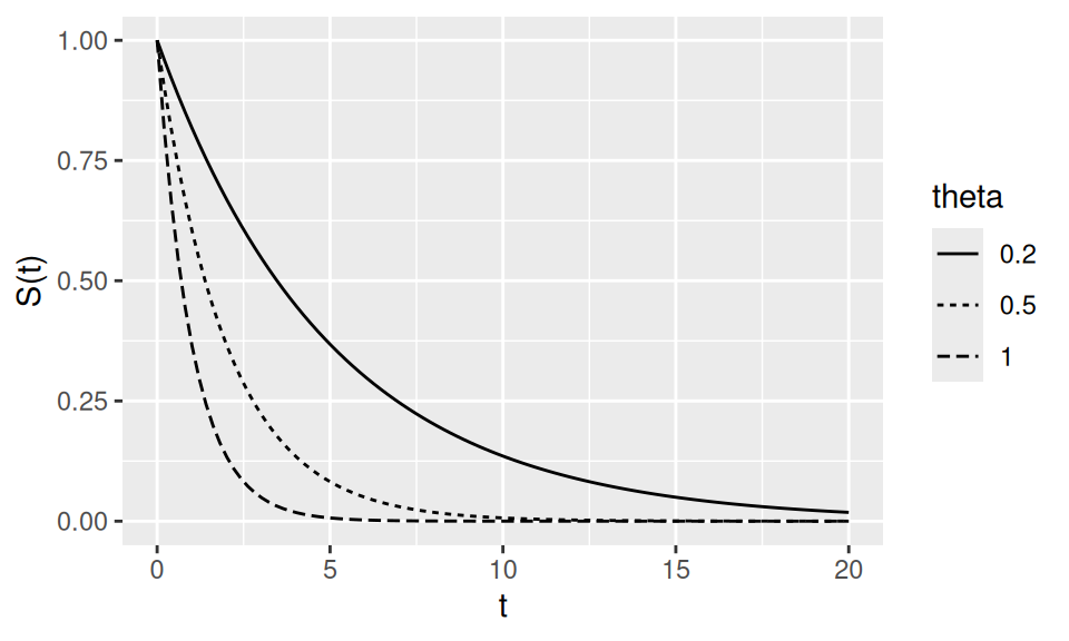
Figure 3.2: \(S(t)\) for \(\theta = 0.2, 0.5, 1\).
Assuming the mean survival time to be \(100\) days for a fatal late detected cancer, we can expect that half of the patients survive \(69.3\) days after chemo since
## [1] 69.31472You will learn more about this in a third-year module, MATH3085: Survival Models, which is important in the actuarial profession.
3.5.2.5 Memoryless property
Like the geometric distribution, the exponential distribution is memoryless: conditional on surviving to time \(t\), the distribution of the additional lifetime is the same as at time 0.
The proof is exactly as in the case of the geometric distribution, reproduced below. Recall the definition of conditional probability: \[P\{A \mid B\}=\frac{P\{A \cap B\}}{P\{B\}}.\] Now the proof, \[\begin{align*} P(X>s+t \mid X>t) &=\frac{P(X>s+t, X>t)}{P(X>t)} \\ &=\frac{P(X>s+t)}{P(X>t)} \\ &=\frac{e^{-\theta(s+t)}}{e^{-\theta t}} \\ &=e^{-\theta s} \\ &=P(X>s). \end{align*}\] Note that the event \(X>s+t\) and \(X>t\) implies and is implied by \(X>s+t\) since \(s>0\).
Example 3.15 Suppose the time \(T\) between any two successive arrivals in a hospital emergency department has exponential distribution, \(T \sim \operatorname{Exponential}(\lambda)\). Historically, the mean of these inter-arrival times is 5 minutes. Estimate \(\lambda\), and hence estimate
- \(P(0<T< 5)\),
- \(P(T<10 \mid T>5)\).
An estimate of \(E(T)\) is 5. As \(E(T)=\frac{1}{\lambda}\) we take \(\frac{1}{5}\) as the estimate of \(\lambda\).
- \(P(0<T<5)=\int_0^5 \frac{1}{5} e^{-t / 5} d t=\left[-e^{-t / 5}\right]_0^5=1-e^{-1}=0.63212\).
- We have \[\begin{align*} P(T<10 \mid T>5) &=\frac{P(5<T<10)}{P(T>5)} \\ &=\frac{\int_5^{10} \frac{1}{5} e^{-t / 5} d t}{\int_5^{\infty} \frac{1}{5} e^{-t / 5} d t}=\frac{\left[-e^{-t / 5}\right]_5^{10}}{\left[-e^{-t / 5}\right]_5^{\infty}} \\ &=1-e^{-1}=0.63212 . \end{align*}\]
3.5.3 Normal distribution
3.5.3.1 Definition
A random variable \(X\) is said to have the normal distribution with parameters \(\mu\) and \(\sigma^2\) if it has pdf of the form \[\begin{equation} f(x)=\frac{1}{\sqrt{2 \pi \sigma^2}} \exp \left\{-\frac{(x-\mu)^2}{2 \sigma^2}\right\}, \; -\infty<x<\infty \tag{3.1} \end{equation}\] where \(-\infty<\mu<\infty\) and \(\sigma>0\) are two given constants. We write \(X \sim N\left(\mu, \sigma^2\right)\).
Later we show \(E(X)=\mu\) and \(\operatorname{Var}(X)=\sigma^2\).
The density (pdf) is much easier to remember and work with when the mean \(\mu=0\) and variance \(\sigma^2=1\). This special case is called the standard normal distribution. In this case, we simply write: \[f(x)=\frac{1}{\sqrt{2 \pi}} \exp \left\{-\frac{x^2}{2}\right\}.\] We often use \(Z\) to denote a random variable with standard normal distribution.
It is easy to see that \(f(x)>0\) for all \(x\). Next, we show \(\int_{-\infty}^{\infty} f(x) d x=1\) or total probability equals 1, so that \(f(x)\) defines a valid pdf:
\[\begin{align*} \int_{-\infty}^{\infty} f(x) d x &=\int_{-\infty}^{\infty} \frac{1}{\sqrt{2 \pi \sigma^2}} \exp \left\{-\frac{(x-\mu)^2}{2 \sigma^2}\right\} d x \\ &=\frac{1}{\sqrt{2 \pi}} \int_{-\infty}^{\infty} \exp \left\{-\frac{z^2}{2}\right\} d z \quad \text { (substitute } z=\frac{x-\mu}{\sigma} \text { so that } d x=\sigma d z) \\ &=\frac{1}{\sqrt{2 \pi}} 2 \int_0^{\infty} \exp \left\{-\frac{z^2}{2}\right\} d z \quad \text { (since the integrand is an even function) } \\ &=\frac{1}{\sqrt{2 \pi}} 2 \int_0^{\infty} \exp \{-u\} \frac{d u}{\sqrt{2 u}}\text { (substitute } u=\frac{z^2}{2} \text { so that } z=\sqrt{2 u} \text { and } d z=\frac{d u}{\sqrt{2 u}}) \\ &=\frac{1}{2 \sqrt{\pi}} 2 \int_0^{\infty} u^{\frac{1}{2}-1} \exp \{-u\} d u \quad \text { (rearrange the terms) } \\ &=\frac{1}{\sqrt{\pi}} \Gamma\left(\frac{1}{2}\right) \quad \text { (recall the definition of the Gamma function) }\\ &=\frac{1}{\sqrt{\pi}} \sqrt{\pi}=1 \quad \text { as } \Gamma\left(\frac{1}{2}\right)=\sqrt{\pi}. \end{align*}\]
3.5.3.2 Linear transformations
Theorem 3.8 If \(X \sim N(\mu,\sigma^2)\) and \(Y=aX+b\), then \(Y \sim N(a\mu+b, a^2\sigma^2)\).
Proof. The cumulative distribution function of \(Y\) is \[\begin{align*} F_Y(y) &= P(Y \leq y) = P(aX + b \leq y) = P\left(X \leq \frac{y-b}{a}\right) \\ &= \int_{-\infty}^{\frac{y-b}{a}} f_X(x) dx, \text{ where $f_X(x)$ is the pdf of $X$} \\ &= \int_{-\infty}^y \frac{1}{a} f_X\left(\frac{u-b}{a}\right) du, \text{ substituting $u = ax + b$.} \end{align*}\]
So \(Y\) has probability density function \[\begin{align*} f_Y(y) &= \frac{1}{a} f_X\left(\frac{y-b}{a}\right) \\ &= \frac{1}{a} \frac{1}{\sqrt{2 \pi \sigma^2}} \exp\left\{-\frac{\left(\frac{y-b}{a} - \mu\right)^2}{2 \sigma^2}\right\} \\ &= \frac{1}{\sqrt{2 \pi a^2 \sigma^2}} \exp\left\{-\frac{\left(y-b - a\mu\right)^2}{2 a^2 \sigma^2}\right\}, \end{align*}\] which is the \(N(a \mu + b, a^2 \sigma^2)\) probability density function. So \(Y \sim N(a \mu + b, a^2 \sigma^2)\).
An important consequence is that if \(X \sim N(\mu, \sigma^2)\), then \(Z = (X-\mu)/\sigma \sim N(0, 1)\). We can “standardise” any normal random variable by subtracting the mean \(\mu\) then dividing by the standard deviation \(\sigma\).
3.5.3.3 Expectation and variance
We claimed that \(E(X)=\mu\) and \(\operatorname{Var}(X)=\sigma^2\), and now will prove these results.
\(E(X)=\mu\) because \(f(x)\) is symmetric about \(\mu\).
To prove \(\operatorname{Var}(X)=\sigma^2\), we show that \(\operatorname{Var}(Z)=1\) where \(Z=\frac{X-\mu}{\sigma}\). Once we have shown that, we will have \(\operatorname{Var}(X)=\sigma^2 \operatorname{Var}(Z)=\sigma^2\).
Since \(E(Z)=0, \operatorname{Var}(Z)=E\left(Z^2\right)\), which is calculated below: \[\begin{align*} E\left(Z^2\right) &=\int_{-\infty}^{\infty} z^2 f(z) d z \\ &=\int_{-\infty}^{\infty} z^2 \frac{1}{\sqrt{2 \pi}} \exp \left\{-\frac{z^2}{2}\right\} d z \\ &=\frac{2}{\sqrt{2 \pi}} \int_0^{\infty} z^2 \exp \left\{-\frac{z^2}{2}\right\} d z \quad \text { (since the integrand is an even function) } \\ &=\frac{2}{\sqrt{2 \pi}} \int_0^{\infty} 2 u \exp \{-u\} \frac{d u}{\sqrt{2 u}} \quad \text { (substitute } u=\frac{z^2}{2} \text { so that } z=\sqrt{2 u} \text { and } d z=\frac{d u}{\sqrt{2 u}} ) \\ &=\frac{4}{2 \sqrt{\pi}} \int_0^{\infty} u^{\frac{1}{2}} \exp \{-u\} d u \\ &=\frac{2}{\sqrt{\pi}} \int_0^{\infty} u^{\frac{3}{2}}-1 \exp \{-u\} d u \\ &=\frac{2}{\sqrt{\pi}} \Gamma\left(\frac{3}{2}\right) \quad \text { (definition of the gamma function) }\\ &=\frac{2}{\sqrt{\pi}}\left(\frac{3}{2}-1\right) \Gamma\left(\frac{3}{2}-1\right) \quad \text { (reduction property of the gamma function) }\\ &=\frac{2}{\sqrt{\pi}} \frac{1}{2} \sqrt{\pi} \quad\text { (since } \Gamma\left(\frac{1}{2}\right) =\sqrt{\pi}) \\ &=1, \end{align*}\] as we hoped for! This proves \(\operatorname{Var}(X)=\sigma^2\).
3.5.3.4 Calculating probabilities
Suppose \(X \sim N\left(\mu, \sigma^2\right)\) and we are interested in finding \(P(a \leq X \leq b)\) for two constants \(a\) and \(b\). To do this, we can use the fact that \(Z = \frac{X - \mu}{\sigma} \sim N(0, 1)\) and rewrite the probability of interest in terms of standard normal probabilities: \[\begin{align*} P(a \leq X \leq b) &= P\left(\frac{a-\mu}{\sigma} \leq Z \leq \frac{b-\mu}{\sigma}\right) \\ &=P\left(Z \leq \frac{b-\mu}{\sigma}\right)- P\left(Z \leq \frac{a-\mu}{\sigma}\right) \\ &=\Phi\left(\frac{b-\mu}{\sigma}\right)-\Phi\left(\frac{a-\mu}{\sigma}\right), \end{align*}\] where we use the notation \(\Phi(\cdot)\) to denote the cdf of the standard normal distribution, i.e. \[\Phi(z)= P(Z \leq z)=\int_{-\infty}^z \frac{1}{\sqrt{2 \pi}} \exp \left\{-\frac{u^2}{2}\right\} d u.\] This result allows us to find the probabilities about a normal random variable \(X\) of any mean \(\mu\) and variance \(\sigma^2\) through the probabilities of the standard normal random variable \(Z\). For this reason, only \(\Phi(z)\) is tabulated. Further more, due to the symmetry of the pdf of \(Z, \Phi(z)\) is tabulated only for positive \(z\) values. Suppose \(a>0\), then \[\begin{align*} \Phi(-a)=P(Z \leq-a) &=P(Z>a) \\ &=1-P(Z \leq a) \\ &=1-\Phi(a). \end{align*}\]
In R, pnorm computes normal cdf values with arguments mean (for \(\mu\)) and sd (for \(\sigma\)). Defaults are mean = 0, sd = 1 (standard normal).
So, we use the command
## [1] 0.8413447to calculate \(\Phi(1)=P(Z \leq 1)\). We can also use the command
## [1] 0.9937903to calculate \(P(X \leq 15)\) when \(X \sim N\left(\mu=10, \sigma^2=4\right)\) directly.
- \(P(-1<Z<1)=\Phi(1)-\Phi(-1)=0.6827\). This means that \(68.27 \%\) of the probability lies within 1 standard deviation of the mean.
- \(P(-2<Z<2)=\Phi(2)-\Phi(-2)=0.9545\). This means that \(95.45 \%\) of the probability lies within 2 standard deviations of the mean.
- \(P(-3<Z<3)=\Phi(3)-\Phi(-3)=0.9973\). This means that \(99.73 \%\) of the probability lies within 3 standard deviations of the mean.
We are often interested in the quantiles (inverse-cdf of probability), \(\Phi^{-1}(\cdot)\) of the normal distribution for various reasons. We find the \(p\)th quantile by issuing the R command qnorm(p)
- \(\texttt{qnorm(0.95)} = \Phi^{-1}(0.95) = 1.645\). This means that the 95th percentile of the standard normal distribution is 1.645. This also means that \(P(-1.645<Z<1.645)=\Phi(1.645)-\) \(\Phi(-1.645)=0.90\).
- \(\texttt{qnorm(0.975)} = \Phi^{-1}(0.975) = 1.96\). This means that the 97.5th percentile of the standard normal distribution is 1.96. This also means that \(P (-1.96 < Z < 1.96) = \Phi(1.96) - \Phi(-1.96) = 0.95\).
Example 3.16 Suppose the marks in MATH1063 follow the normal distribution with mean 58 and standard deviation 32.25.
- What percentage of students will fail (i.e. score less than 40) in MATH1063?
Answer: \(\texttt{pnorm(40, mean=58, sd=32.25)} = 28.84\%\). - What percentage of students will get an A result (score greater than 70)?
Answer: \(\texttt{1 - pnorm(70, mean=58, sd=32.25)} = 35.49\%\). - What is the probability that a randomly selected student will score more than 90?
Answer: \(\texttt{1 - pnorm(90, mean=58, sd=32.25)} = 0.1605\). - What is the probability that a randomly selected student will score less than 25?
Answer: \(\texttt{pnorm(25, mean=58, sd=32.25) = 0.1531}\). - What is the probability that a randomly selected student scores a 2:1 (i.e. a mark between 60 and 70)? Left as an exercise.
Example 3.17 A lecturer set and marked an examination and found that the distribution of marks was \(N (42, 14^2 )\). The school’s policy is to present scaled marks whose distribution is \(N (50, 15^2 )\). What linear transformation should the lecturer apply to the raw marks to accomplish this and what would the raw mark of 40 be transformed to?
Let \(X\) be the raw mark and \(Y\) the scaled mark. We have \(X \sim N (\mu_x = 42, \sigma_x^2 = 14^2 )\) and aim to define the scaling such that \(Y \sim N (\mu_y = 50, \sigma_y^2 = 15^2)\). If we standardise both variables, they should each have standard normal distribution, so we choose \(Y\) such that \[\frac{X - \mu_x}{\sigma_x} = \frac{Y - \mu_y}{\sigma_y}\] giving \[Y = \mu_y + \frac{\sigma_y}{\sigma_x}(X - \mu_x) = 50 + \frac{15}{14}(X - 42).\]
Now at raw mark \(X = 40\), the transformed mark would be \[Y = 50 + \frac{15}{14}(40 - 42) = 47.86.\]
3.5.3.5 Log-normal distribution
If \(X \sim N(\mu,\sigma^2)\) and \(Y=\exp(X)\), then \(Y\) is log-normal with parameters \(\mu\) and \(\sigma^2\).
The mean of the random variable \(Y\) is given by \[\begin{align*} E(Y) &=E[\exp (X)] \\ &=\int_{-\infty}^{\infty} \exp (x) \frac{1}{\sigma \sqrt{2 \pi}} \exp \left\{-\frac{(x-\mu)^2}{2 \sigma^2}\right\} d x \\ &=\exp \left\{-\frac{\mu^2-\left(\mu+\sigma^2\right)^2}{2 \sigma^2}\right\} \int_{-\infty}^{\infty} \frac{1}{\sigma \sqrt{2 \pi}} \exp \left\{-\frac{x^2-2\left(\mu+\sigma^2\right) x+\left(\mu+\sigma^2\right)^2}{2 \sigma^2}\right\} d x \\ &=\exp \left\{-\frac{\mu^2-\left(\mu+\sigma^2\right)^2}{2 \sigma^2}\right\} \quad \text{(integrating a $N(\mu+\sigma^2, \sigma^2)$ random variable over its domain) }\\ &=\exp \left\{\mu+\sigma^2 / 2\right\}. \end{align*}\] Similarly, one can show that \[\begin{align*} E(Y^2) &=E[\exp (2 X)] \\ &=\int_{-\infty}^{\infty} \exp (2 x) \frac{1}{\sigma \sqrt{2 \pi}} \exp \left\{-\frac{(x-\mu)^2}{2 \sigma^2}\right\} d x \\ &=\cdots \\ &=\exp \left\{2 \mu+2 \sigma^2\right\}. \end{align*}\] Hence, the variance is given by \[\operatorname{Var}(Y)=E(Y^2)-(E(Y))^2=\exp \left\{2 \mu+2 \sigma^2\right\}-\exp \left\{2 \mu+\sigma^2\right\}.\]
The log-normal distribution is often used in practice for modelling economic variables of interest in business and finance, e.g. volume of sales, income of individuals. You do not need to remember the mean and variance of the log-normal distribution.
3.6 Joint distributions
3.6.1 Introduction
We often study multiple random variables together (e.g., height and weight) to exploit relationships between them. Joint probability distributions provide the framework. We introduce covariance, correlation, and independence.
3.6.2 Joint distribution of discrete random variables
For discrete \(X\) and \(Y\), \(f(x,y)=P(X=x, Y=y)\) is the joint probability mass function (pmf). It must satisfy: \[f (x, y) \geq 0 \quad \text{ for all $x$ and $y$}\] and \[\sum_{\text{all $x$}} \sum_{\text{all $y$}} f(x, y) = 1.\] The marginal probability mass functions (marginal pmfs) of \(X\) and \(Y\) are respectively \[f_X(x) = \sum_y f(x, y), \quad f_Y(y) = \sum_x f(x, y)\] Use the identity \(\sum_{x} \sum_{y} f(x, y) = 1\) to prove that \(f_X(x)\) and \(f_Y(y)\) are really pmfs.
Example 3.18 Suppose that two fair dice are tossed independently one after the other. Let \[X = \begin{cases} -1 & \text{if the result from die 1 is larger} \\ 0 & \text{if the results are equal} \\ 1 & \text{if the result from die 1 is smaller} \end{cases} \] and let \(Y = |\text{difference between the two dice}|\). Find the joint probability pmf for \(X\) and \(Y\).
There are 36 possible outcomes for the results of the dice rolls, and each gives a pair of values \((x, y)\) for \(X\) and \(Y\).
| 1 | 2 | 3 | 4 | 5 | 6 | |
|---|---|---|---|---|---|---|
| 1 | (0, 0) | (1, 1) | (1, 2) | (1, 3) | (1, 4) | (1, 5) |
| 2 | (-1, 1) | (0, 0) | (1, 1) | (1, 2) | (1, 3) | (1, 4) |
| 3 | (-1, 2) | (-1, 1) | (0, 0) | (1, 1) | (1, 2) | (1, 3) |
| 4 | (-1, 3) | (-1, 2) | (-1, 1) | (0, 0) | (1, 1) | (1, 2) |
| 5 | (-1, 4) | (-1, 3) | (-1, 2) | (-1, 1) | (0, 0) | (1, 1) |
| 6 | (-1, 5) | (-1, 4) | (-1, 3) | (-1, 2) | (-1, 1) | (0, 0) |
The joint pmf is given in Table ??.
| $y$ | ||||||
| $x$ | 0 | 1 | 2 | 3 | 4 | 5 |
|---|---|---|---|---|---|---|
| -1 | $\frac{0}{36}$ | $\frac{5}{36}$ | $\frac{4}{36}$ | $\frac{3}{36}$ | $\frac{2}{36}$ | $\frac{1}{36}$ |
| 0 | $\frac{6}{36}$ | $\frac{0}{36}$ | $\frac{0}{36}$ | $\frac{0}{36}$ | $\frac{0}{36}$ | $\frac{0}{36}$ |
| 1 | $\frac{0}{36}$ | $\frac{5}{36}$ | $\frac{4}{36}$ | $\frac{3}{36}$ | $\frac{2}{36}$ | $\frac{1}{36}$ |
The marginal pmf for \(X\) is \[f_X(x) = \begin {cases} \frac{15}{36} & \text{if $x = -1$} \\ \frac{6}{36} & \text{if $x = 0$} \\ \frac{15}{36} & \text{if $x = 1$.} \end{cases}\]
Exercise: Write down the marginal distribution of \(Y\) and hence find the mean and variance of \(Y\).
3.6.3 Joint distribution of continuous random variables
For continuous \(X\) and \(Y\), a nonnegative function \(f(x,y)\) is a joint pdf if \[\int_{-\infty}^{\infty} \int_{-\infty}^{\infty} f(x, y) d x \, d y=1\] The marginal pdfs of \(X\) and \(Y\) are respectively \[f_X(x)=\int_{-\infty}^{\infty} f(x, y) d y, \quad f_Y(y)=\int_{-\infty}^{\infty} f(x, y) d x\]
Example 3.19 Define a joint pdf by \[f(x, y)= \begin{cases} 6 x y^2 & \text { if $0<x<1$ and $0<y<1$} \\ 0 & \text { otherwise. } \end{cases}\] How can we show that the above is a pdf? It is non-negative for all \(x\) and \(y\) values. But does it integrate to 1? We are going to use the following rule.
Result: Suppose that a real-valued function \(f(x, y)\) is continuous in a region \(A\), where \(A = \{(x, y) \text{ such that } a<x<b \text{ and } c<y<d\}\). Then \[\int_A f(x, y) d x d y=\int_c^d \int_a^b f(x, y) d x \, dy.\] The same result holds if \(a\) and \(b\) depend upon \(y\), but \(c\) and \(d\) should be free of \(x\) and \(y\). When we evaluate the inner integral \(\int_a^b f(x, y) d x\), we treat \(y\) as constant.
Notes: To evaluate a bivariate integral over a region \(A\) we:
- Draw a picture of \(A\) whenever possible.
- Rewrite the region \(A\) as an intersection of two one-dimensional intervals. The first interval is obtained by treating one variable as constant.
- Perform two one-dimensional integrals.
Example 3.20 Continuing Example 3.19, \[\begin{align*} \int_0^1 \int_0^1 f(x, y) d x d y &=\int_0^1 \int_0^1 6 x y^2 d x d y \\ &=6 \int_0^1 y^2 d y \int_0^1 x d x \\ &=3 \int_0^1 y^2 d y\left[\text { as } \int_0^1 x d x=\frac{1}{2}\right] \\ &=1 .\left[\text { as } \int_0^1 y^2 d y=\frac{1}{3}\right] \end{align*}\] Now we can find the marginal pdfs as well. \[f_X(x)=2 x, \, 0<x<1, \quad f_Y(y)=3 y^2, \, 0<y<1.\]
The probability of any event in the two-dimensional space can be found by integration and again more details will be provided in the second-year module Statistical Inference.
3.6.4 Covariance and correlation
We first define the expectation of a real-valued scalar function \(g(X, Y)\) of \(X\) and \(Y\) : \[E[g(X, Y)]= \begin{cases}\sum_x \sum_y g(x, y) f(x, y) & \text { if } X \text { and } Y \text { are discrete } \\ \int_{-\infty}^{\infty} \int_{-\infty}^{\infty} g(x, y) f(x, y) d x d y & \text { if } X \text { and } Y \text { are continuous. }\end{cases}\]
Example 3.21 Continuing Example 3.18, let \(g(x, y)=x y\). \[E(X Y)=(-1)(0) 0+(-1)(1) \frac{5}{36}+\cdots+(1)(5) \frac{1}{36}=0.\] Exercises: Try \(g(x, y)=x\). It will be the same thing as \(E(X)=\sum_x x f_X(x)\).
We will not consider any continuous examples as the second-year module Statistical Inference will study them in detail.
Suppose that two random variables \(X\) and \(Y\) have joint pmf or pdf \(f(x, y)\) and let \(E(X)=\mu_x\) and \(E(Y)=\mu_y\). The covariance between \(X\) and \(Y\) is defined by \[\operatorname{Cov}(X, Y)=E\left[\left(X-\mu_x\right)\left(Y-\mu_y\right)\right]=E(X Y)-\mu_x \mu_y.\] Let \(\sigma_x^2=\operatorname{Var}(X)=E\left(X^2\right)-\mu_x^2\) and \(\sigma_y^2=\operatorname{Var}(Y)=E\left(Y^2\right)-\mu_y^2\). The correlation coefficient between \(X\) and \(Y\) is defined by: \[\operatorname{Corr}(X, Y)=\frac{\operatorname{Cov}(X, Y)}{\sqrt{\operatorname{Var}(X) \operatorname{Var}(Y)}}=\frac{E(X Y)-\mu_x \mu_y}{\sigma_x \sigma_y}.\] It can be proved that for any two random variables, \(-1 \leq \operatorname{Corr}(X, Y) \leq 1\). The correlation \(\operatorname{Corr}(X, Y)\) is a measure of linear dependency between two random variables \(X\) and \(Y\), and it is free of the measuring units of \(X\) and \(Y\) as the units cancel in the ratio.
3.6.5 Independence
Two events \(A\) and \(B\) are independent if \(P(A\cap B)=P(A)P(B)\). Analogously, random variables \(X\) and \(Y\) with joint pmf/pdf \(f(x,y)\) are independent iff \(f(x,y)=f_X(x)f_Y(y)\) for all \(x,y\).
In the discrete case \(X\) and \(Y\) are independent if each cell probability, \(f(x, y)\), is the product of the corresponding row and column totals. In Example 3.18 \(X\) and \(Y\) are not independent.
Example 3.22 Suppose \(X\) and \(Y\) have joint pdf given by the probability table:
| \(y\) | |||||
|---|---|---|---|---|---|
| 1 | 2 | 3 | Total | ||
| \(x\) | 0 | \(\frac{1}{6}\) | \(\frac{1}{12}\) | \(\frac{1}{12}\) | \(\frac{1}{3}\) |
| 1 | \(\frac{1}{4}\) | \(\frac{1}{8}\) | \(\frac{1}{8}\) | \(\frac{1}{2}\) | |
| 2 | \(\frac{1}{12}\) | \(\frac{1}{24}\) | \(\frac{1}{24}\) | \(\frac{1}{6}\) | |
| Total | \(\frac{1}{2}\) | \(\frac{1}{4}\) | \(\frac{1}{4}\) | 1 |
Verify that in the following example \(X\) and \(Y\) are independent. We need to check all 9 cells.
Example 3.23 Let \(f(x, y)=6 x y^2, 0<x<1,0<y<1\). Check that \(X\) and \(Y\) are independent.
Example 3.24 Let \(f(x, y)=2 x, 0 \leq x \leq 1,0 \leq y \leq 1\). Check that \(X\) and \(Y\) are independent.
Sometimes the joint pdf may look like something you can factorise, but \(X\) and \(Y\) may not be independent because they may be related in the domain. For instance,
- \(f(x, y)=\frac{21}{4} x^2 y, x^2 \leq y \leq 1\). Not independent!
- \(f(x, y)=e^{-y}, 0<x<y<\infty\). Not independent!
Here are some useful consequences of independence:
- Suppose that \(X\) and \(Y\) are independent random variables. Then \[P(X \in A, Y \in B)=P(X \in A) \times P(Y \in B)\] for any events \(A\) and \(B\). That is, the joint probability can be obtained as the product of the marginal probabilities. We will use this result in the next section. For example, suppose Jack and Jess are two randomly selected students. Let \(X\) denote the height of Jack and \(Y\) denote the height of Jess. Then \[P(X<182 \text { and } Y>165)=P(X<182) \times P(Y>165) .\] This holds for any thresholds and inequalities.
- Let \(g(x)\) be a function of \(x\) only and \(h(y)\) be a function of \(y\) only. Then, if \(X\) and \(Y\) are independent, \[E[g(X) h(Y)]=E[g(X)] \times E[h(Y)].\] As a special case, let \(g(x)=x\) and \(h(y)=y\). Then we have \[E(X Y)=E(X) \times E(Y).\] Consequently, for independent random variables \(X\) and \(Y, \operatorname{Cov}(X, Y)=0\) and \(\operatorname{Corr}(X, Y)=\) 0. But the converse is not true in general. That is, merely having \(\operatorname{Corr}(X, Y)=0\) does not imply that \(X\) and \(Y\) are independent random variables.
3.7 Sums of random variables
Sums of random variables appear frequently in practice and theory. For example, an exam mark is the sum of question scores, and the sample mean is proportional to a sum.
Suppose we have obtained a random sample from a distribution with pmf or pdf \(f(x)\), so that \(X\) can either be a discrete or a continuous random variable. We will learn more about random sampling in the next chapter. Let \(X_1, \ldots, X_n\) denote the random sample of size \(n\) where \(n\) is a positive integer. We use upper case letters since each member of the random sample is a random variable. For example, I toss a fair coin \(n\) times and let \(X_i\) take the value 1 if a head appears in the \(i\) th trial and 0 otherwise. Now I have a random sample \(X_1, \ldots, X_n\) from the Bernoulli distribution with probability of success equal to \(0.5\) since the coin is assumed to be fair.
We can get a random sample from a continuous random variable as well. Suppose it is known that the distribution of the heights of first-year students is normal with mean 175 centimetres and standard deviation 8 centimetres. I can randomly select a number of first-year students and record each student’s height.
Suppose \(X_1, \ldots, X_n\) is a random sample from a population with distribution \(f(x)\). Then it can be shown that the random variables \(X_1, \ldots, X_n\) are mutually independent, i.e. \[P\left(X_1 \in A_1, X_2 \in A_2, \ldots, X_n \in A_n\right)=P\left(X_1 \in A_1\right) \times P\left(X_2 \in A_2\right) \times \cdots P\left(X_n \in A_n\right)\] for any set of events, \(A_1, A_2, \ldots A_n\). That is, the joint probability can be obtained as the product of individual probabilities. An example of this for \(n=2\) was given in Section 3.6.5.
Example 3.25 (Distribution of the sum of independent binomial random variables) Suppose \(X \sim \operatorname{Bin}(m, p)\) and \(Y \sim \operatorname{Bin}(n, p)\) independently. Note that \(p\) is the same in both distributions. Using the above fact that joint probability is the multiplication of individual probabilities, we can conclude that \(Z=X+Y\) has the binomial distribution. It is intuitively clear that this should happen since \(X\) comes from \(m\) Bernoulli trials and \(Y\) comes from \(n\) Bernoulli trials independently, so \(Z\) comes from \(m+n\) Bernoulli trials with common success probability \(p\).
Next we will prove the result mathematically, by finding the probability mass function of \(Z=X+Y\) directly and observing that it is of the appropriate form. In our proof, we will need to use the fact that \[\sum_{x+y=z} \binom{m}{x}\binom{n}{y} = \binom{m+n}{z}\] where the above sum is also over all possible integer values of \(x\) and \(y\) such that \(0 \leq x \leq m\) and \(0 \leq y \leq n\). This fact may be proved by using the binomial theorem, but we state it here without proof.
Note that \[P(Z=z)=P(X=x, Y=y)\] subject to the constraint that \(x+y=z\), \(0 \leq x \leq m\), \(0 \leq y \leq n\). Thus, \[\begin{align*} P(Z=z) &= \sum_{x+y=z} P(X=x, Y=y) \\ &= \sum_{x+y=z} \binom{m}{x} p^x(1-p)^{m-x}\binom{n}{y} p^y(1-p)^{n-y} \\ &= \sum_{x+y=z} \binom{m}{x}\binom{n}{y} p^z(1-p)^{m+n-z} \\ &= p^z(1-p)^{m+n-z} \sum_{x+y=z} \binom{m}{x}\binom{n}{y} \\ &= \binom{m+n}{z} p^z(1-p)^{m+n-z}, \; \; \text{using the fact above.} \end{align*}\] Thus, we have proved that the sum of independent binomial random variables with common probability is binomial as well. This is called the reproductive property of random variables.
Now we will state two main results without proof. The proofs will presented in the second-year Statistical Inference. Suppose that \(X_1, \ldots, X_n\) is a random sample from a population distribution with finite variance, and suppose that \(E\left(X_i\right)=\mu_i\) and \(\operatorname{Var}\left(X_i\right)=\sigma_i^2\). Define a new random variable \[Y=X_1+ X_2+\cdots+ X_n.\] Then:
- \(E(Y)=\mu_1+\mu_2+\cdots+ \mu_n\).
- \(\operatorname{Var}(Y)=\sigma_1^2+ \sigma_2^2+\cdots+ \sigma_n^2\).
That is:
- The expectation of the sum of independent random variables is the sum of the expectations of the individual random variables
- the variance of the sum of independent random variables is the sum of the variances of the individual random variables.
The second result is only true for independent random variables, e.g. random samples. Now we will consider many examples.
Example 3.26 (Mean and variance of binomial distribution) Suppose \(Y \sim \operatorname{Bin}(n, p)\). Then we can write: \[Y=X_1+X_2+\ldots+X_n\] where each \(X_i\) is an independent Bernoulli trial with success probability \(p\). We have shown before that, \(E\left(X_i\right)=p\) and \(\operatorname{Var}\left(X_i\right)=p(1-p)\) by direct calculation. Now the above two results imply that: \[ E(Y)=E\left(\sum_{i=1}^n X_i\right)=p+p+\ldots+p=n p . \\ \operatorname{Var}(Y)=\operatorname{Var}\left(X_1\right)+\cdots+\operatorname{Var}\left(X_n\right)=p(1-p)+\ldots+p(1-p)=n p(1-p) . \] Thus we avoided the complicated sums used to derive \(E(X)\) and \(\operatorname{Var}(X)\) in Sections 3.4.2.3 and 3.4.2.4.
Example 3.27 (Mean and variance of negative binomial distribution) Recall that the negative binomial random variable \(Y\) is the number of trials needed to obtain the \(r\)th success in a sequence of independent Bernoulli trials, each with success probability \(p\). Let \(X_i\) be the number of trials needed after the \((i-1)\)th success to obtain the \(i\)th success. Each \(X_i\) is a geometric random variable and \(Y=X_1+\cdots+X_r\). Hence \[E(Y)=E(X_1)+\cdots+E(X_r)=1 / p+\cdots+1 / p=r / p\] and \[\operatorname{Var}(Y)=\operatorname{Var}(X_)+\cdots+\operatorname{Var}(X_r)=(1-p) / p^2+\cdots+(1-p) / p^2=r(1-p) / p^2.\]
Example 3.28 (Sum of independent normal random variables) Suppose that \(X_i \sim N\left(\mu_i, \sigma_i^2\right), i=1,2, \ldots, k\) are independent random variables. Suppose that \[Y=a_1 X_1+\cdots+a_k X_k.\] Then we can prove that: \[Y \sim N\left(\sum_{i=1}^k \mu_i, \sum_{i=1}^k \sigma_i^2\right).\] It is clear that \(E(Y)=\sum_{i=1}^k \mu_i\) and \(\operatorname{Var}(Y)=\sum_{i=1}^k \sigma_i^2\). But that \(Y\) has the normal distribution cannot yet be proved with the theory we know. This proof will be provided in the second-year module Statistical Inference.
As a consequence of the stated result we can easily see the following. Suppose \(X_1\) and \(X_2\) are independent \(N\left(\mu, \sigma^2\right)\) random variables. Then \(2 X_1 \sim N\left(2 \mu, 4 \sigma^2\right), X_1+X_2 \sim N\left(2 \mu, 2 \sigma^2\right)\), and \(X_1-X_2 \sim N\left(0,2 \sigma^2\right)\). Note that \(2 X_1\) and \(X_1+X_2\) have different distributions. Suppose that \(X_i \sim N\left(\mu, \sigma^2\right), i=1, \ldots, n\) are independent. Then \[X_1+\cdots+X_n \sim N\left(n \mu, n \sigma^2\right),\] and consequently \[\bar{X}=\frac{1}{n}\left(X_1+\cdots+X_n\right) \sim N\left(\mu, \frac{\sigma^2}{n}\right).\]
3.8 The Central Limit Theorem
3.8.1 Introduction
The Central Limit Theorem (CLT) describes the behaviour of sums (and averages) of independent random variables. It applies broadly: independence and finite means and variances suffice. A version follows.
3.8.2 Statement of the Central Limit Theorem (CLT)
Let \(X_{1}, \ldots, X_{n}\) be independent random variables with finite \(E\left(X_{i}\right)=\mu_{i}\) and finite \(\operatorname{Var}\left(X_{i}\right)=\sigma_{i}^{2}\). Define \(Y=\sum_{i=1}^{n} X_{i}\). Then, for a sufficiently large \(n\), the central limit theorem states that \(Y\) is approximately normally distributed with \[E(Y)=\sum_{i=1}^{n} \mu_{i}, \quad \operatorname{Var}(Y)=\sum_{i=1}^{n} \sigma_{i}^{2}.\] This also implies that \(\bar{X}=\frac{1}{n} Y\) also follows the normal distribution approximately, as the sample size \(n \rightarrow \infty\). In particular, if \(\mu_{i}=\mu\) and \(\sigma_{i}^{2}=\sigma^{2}\), i.e. all means are equal and all variances are equal, then the CLT states that, as \(n \rightarrow \infty\), \[\bar{X} \sim N\left(\mu, \frac{\sigma^{2}}{n}\right).\] Equivalently, \[\frac{\sqrt{n}(\bar{X}-\mu)}{\sigma} \sim N(0,1)\] as \(n \rightarrow \infty\). The notion of convergence is explained by the convergence of distribution of \(\bar{X}\) to that of the normal distribution with the appropriate mean and variance. It means that the \(\mathrm{cdf}\) of the left hand side, \(\sqrt{n} \frac{(\bar{X}-\mu)}{\sigma}\), converges to the cdf of the standard normal random variable, \(\Phi(\cdot)\). In other words, \[\lim _{n \rightarrow \infty} P\left(\sqrt{n} \frac{(\bar{X}-\mu)}{\sigma} \leq z\right)=\Phi(z), \quad-\infty<z<\infty.\] So for “large samples”, we can use \(N(0,1)\) as an approximation to the sampling distribution of \(\sqrt{n}(\bar{X}-\mu) / \sigma\). This result is ‘exact’, i.e. no approximation is required, if the distribution of the \(X_{i}\) ’s are normal in the first place — this was discussed in the previous lecture.
How large must \(n\) be? It depends on how close the \(X_i\) distributions are to normal. The approximation is often reasonable for \(n \approx 20\) (sometimes smaller), but heavy skewness typically requires larger \(n\). We investigate in one example in Figure 3.3.
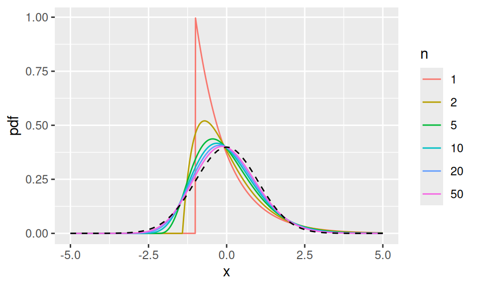
Figure 3.3: Distribution of normalised sample means for samples of different sizes. Initially very skew (original distribution, \(n=1\)) becoming rapidly closer to standard normal (dashed line) with increasing \(n\).
3.8.3 Application of CLT to binomial distribution
We know that a binomial random variable \(Y\) with parameters \(n\) and \(p\) is the number of successes in a set of \(n\) independent Bernoulli trials, each with success probability \(p\). We may write \[Y=X_{1}+X_{2}+\cdots+X_{n},\] where \(X_{1}, \ldots, X_{n}\) are independent Bernoulli random variables with success probability \(p\). It follows from the CLT that, for a sufficiently large \(n, Y\) is approximately normally distributed with expectation \(E(Y)=n p\) and variance \(\operatorname{Var}(Y)=n p(1-p)\).
Hence, for given integers \(y_{1}\) and \(y_{2}\) between 0 and \(n\) and a suitably large \(n\), we have \[\begin{align*} P\left(y_{1} \leq Y \leq y_{2}\right) &=P\left\{\frac{y_{1}-n p}{\sqrt{n p(1-p)}} \leq \frac{Y-n p}{\sqrt{n p(1-p)}} \leq \frac{y_{2}-n p}{\sqrt{n p(1-p)}}\right\} \\ & \approx P\left\{\frac{y_{1}-n p}{\sqrt{n p(1-p)}} \leq Z \leq \frac{y_{2}-n p}{\sqrt{n p(1-p)}}\right\} \end{align*}\] where \(Z \sim N(0,1)\).
Because \(Y\) is integer-valued, apply a continuity correction: replace \([y_1,y_2]\) by \([y_1-0.5,\,y_2+0.5]\) in the normal approximation. \[\begin{align*} P\left(y_{1} \leq Y \leq y_{2}\right) &=P\left(y_{1}-0.5 \leq Y \leq y_{2}+0.5\right) \\ &=P\left\{\frac{y_{1}-0.5-n p}{\sqrt{n p(1-p)}} \leq \frac{Y-n p}{\sqrt{n p(1-p)}} \leq \frac{y_{2}+0.5-n p}{\sqrt{n p(1-p)}}\right\} \\ & \approx P\left\{\frac{y_{1}-0.5-n p}{\sqrt{n p(1-p)}} \leq Z \leq \frac{y_{2}+0.5-n p}{\sqrt{n p(1-p)}}\right\} . \end{align*}\] What do we mean by a suitably large \(n\)? A commonly-used guideline is that the approximation is adequate if \(n p \geq 5\) and \(n(1-p) \geq 5\).
Example 3.29 A producer of natural yoghurt believed that the market share of their brand was \(10 \%\). To investigate this, a survey of 2500 yoghurt consumers was carried out. It was observed that only 205 of the people surveyed expressed a preference for their brand. Should the producer be concerned that they might be losing market share?
Assume that the conjecture about market share is true. Then the number of people \(Y\) who prefer this product follows a binomial distribution with \(p=0.1\) and \(n=2500\). So the mean is \(n p=250\), the variance is \(n p(1-p)=225\), and the standard deviation is 15 . The exact probability of observing \((Y \leq 205)\) is given by the sum of the binomial probabilities up to and including 205, which is difficult to compute. However, this can be approximated by using the CLT: \[\begin{align*} P(Y \leq 205) &=P(Y \leq 205.5) \\ &=P\left\{\frac{Y-n p}{\sqrt{n p(1-p)}} \leq \frac{205.5-n p}{\sqrt{n p(1-p)}}\right\} \\ & \approx P\left\{Z \leq \frac{205.5-n p}{\sqrt{n p(1-p)}}\right\} \\ &=P\left\{Z \leq \frac{205.5-250}{15}\right\} \\ &=\Phi(-2.967)=0.0015. \end{align*}\] This probability is so small that it casts doubt on the validity of the assumption that the market share is \(10 \%\).
Although the exact binomial probabilities are difficult to compute by hand, in this case we may compute them in R. Recall \(Y \sim \operatorname{Bin}(n = 2500, p = 0.1)\), so \(P(Y \leq 205)\) is
## [1] 0.001173725In this case the normal approximation was good enough to correctly conclude that this probability is very small (of the order of \(0.1\%\)), which was all we needed to answer the question of interest here.