Chapter 5 Simple Linear Regression
5.1 What is regression?
So far we have focused on single-variable models, estimating a distribution from random samples of one variable. In many real problems, we want to understand relationships between multiple variables.
Regression models how an “output” variable, the response \(Y\), depends on one or more “input” variables \(x\) (covariates). The response is sometimes called the dependent variable; covariates are also called independent or explanatory variables. In MATH1063 we study simple regression models with a single covariate \(x\).
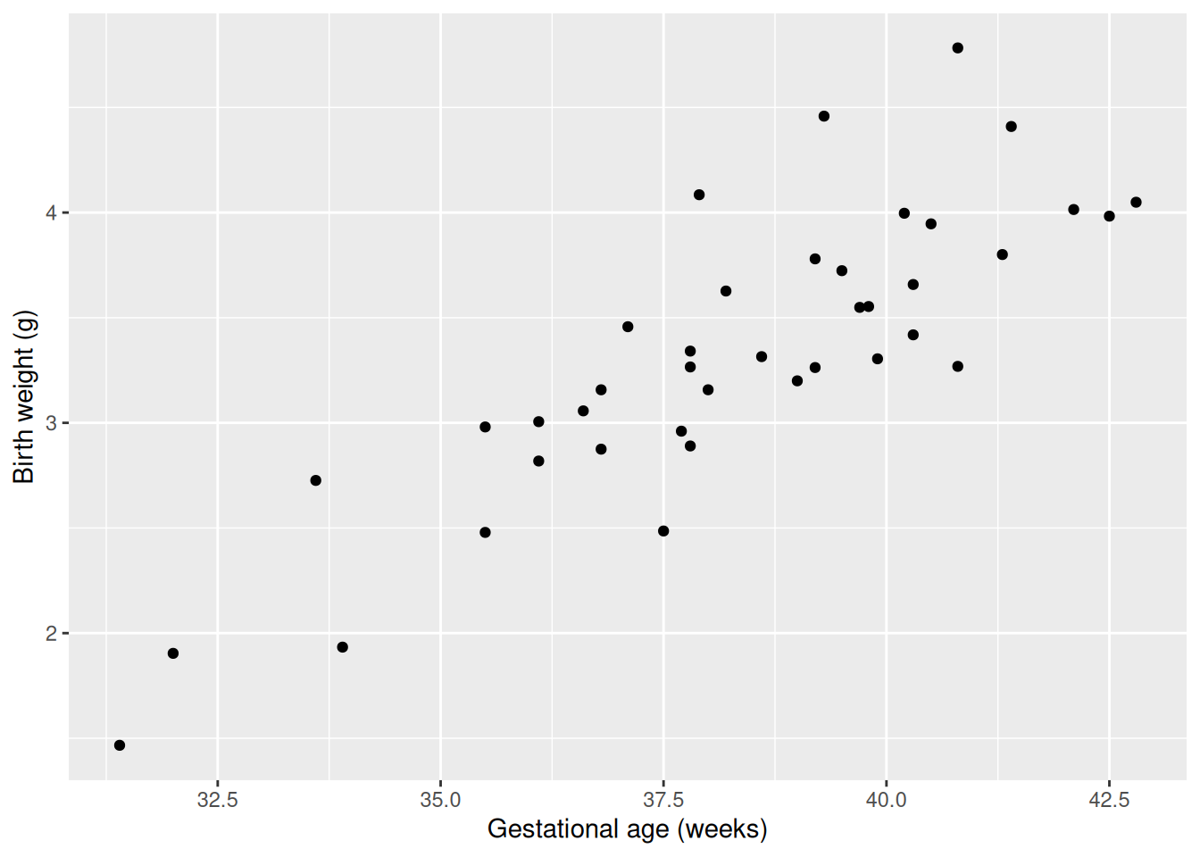
For example, suppose we are interested in how birth weight depends on gestational age (weeks). The response, \(Y\), is birth weight (kg). The covariate, \(x\), is gestational age (weeks). Suppose we have the following data (fictional, but based on real data for male singleton births in Canada).
5.2 Simple linear regression
In simple linear regression, the response depends linearly on the covariate with an additive error: \[Y_i = \beta_0 + \beta_1 x_i + \epsilon_i, \; i = 1, \ldots, n,\] where \(\beta_0\) is the intercept, \(\beta_1\) the slope, and \(\epsilon_i\) a random error. We assume \(\epsilon_i \sim N(0,\sigma^2)\), so the unknown parameters to estimate are \(\beta_0\), \(\beta_1\), and \(\sigma^2\).
We have \[E(Y_i) = \beta_0 + \beta_1 x_i.\] Each choice of \((\beta_0,\beta_1)\) defines a line; these are the regression parameters.
Which line should we choose?
5.3 Estimating the regression parameters
To estimate the unknown regression parameters, we attempt to make the associated straight line as close as possible to the data. We measure the distance between the line and the data with the sum of squares criterion:
\[\text{SS}(\beta_0, \beta_1) = \sum_{i=1}^n (y_i - \beta_0 - \beta_1 x_i)^2.\]
To estimate \(\beta_0\) and \(\beta_1\), we find the values which minimise this sum of squares criterion. These estimates are called the least squares estimates.
To find the least squares estimates, we take partial derivatives of \(SS(\beta_0, \beta_1)\) with respect to \(\beta_0\) and \(\beta_1\), set them to zero, and solve for the parameters.
First, differentiate with respect to \(\beta_0\), to give \[ \frac{\partial SS}{\partial \beta_0} = -2 \sum_{i=1}^n (y_i - \beta_0 - \beta_1 x_i). \] Setting to zero: \[ \sum_{i=1}^n (y_i - \beta_0 - \beta_1 x_i) = 0, \] so \[ n\beta_0 + \beta_1 \sum_{i=1}^n x_i = \sum_{i=1}^n y_i, \] which gives \[ \beta_0 = \bar{y} - \beta_1 \bar{x}. \]
Next, differentiate with respect to \(\beta_1\), to give \[ \frac{\partial SS}{\partial \beta_1} = -2 \sum_{i=1}^n x_i (y_i - \beta_0 - \beta_1 x_i). \] Setting to zero gives \[ \sum_{i=1}^n x_i (y_i - \beta_0 - \beta_1 x_i) = 0, \] or \[ \sum_{i=1}^n x_i y_i - \beta_0 \sum_{i=1}^n x_i - \beta_1 \sum_{i=1}^n x_i^2 = 0. \]
Substituting \(\beta_0 = \bar{y} - \beta_1 \bar{x}\) gives \[ \sum_{i=1}^n x_i y_i - (\bar{y} - \beta_1 \bar{x}) \sum_{i=1}^n x_i - \beta_1 \sum_{i=1}^n x_i^2 = 0, \] so \[ \sum_{i=1}^n x_i y_i - n\bar{y}\bar{x} = \beta_1 \left( \sum_{i=1}^n x_i^2 - n\bar{x}^2 \right). \] So \[ \beta_1 = \frac{\sum_{i=1}^n (x_i - \bar{x})(y_i - \bar{y})}{\sum_{i=1}^n (x_i - \bar{x})^2}. \]
Thus, the least squares estimates are \[ \hat{\beta}_1 = \frac{\sum_{i=1}^n (x_i - \bar{x})(y_i - \bar{y})}{\sum_{i=1}^n (x_i - \bar{x})^2}, \qquad \hat{\beta}_0 = \bar{y} - \hat{\beta}_1 \bar{x}. \]
These estimators are unbiased. The derivation is covered in the second-year module Statistical Modelling I.
5.4 Estimating the variance parameter
We also estimate the error variance \(\sigma^2\).
We estimate \(\sigma^2\) with \[ \hat{\sigma}^2 = \frac{1}{n-2} \sum_{i=1}^n (y_i - \hat{\beta}_0 - \hat{\beta}_1 x_i)^2, \] where \(\hat{\beta}_0\) and \(\hat{\beta}_1\) are the least squares estimates.
This estimator is unbiased for \(\sigma^2\); a derivation appears in Statistical Modelling I.
5.5 Model fitting in R
In practice, we do not need to apply these formulas by hand to find the
least squares estimates. Instead, we can use the lm function in R
to find the estimates. For instance, if the birth weight data is
stored in a data frame called bw, with columns weight for birth weight
(which is the response, \(y\)) and ga for gestational age (which is the covariate, \(x\)),
then we can fit the simple linear regression model with:
We can inspect the fitted model:
##
## Call:
## lm(formula = weight ~ ga, data = bw)
##
## Coefficients:
## (Intercept)           ga
##     -5.1062       0.2203
We see \(\hat \beta_0 =\) -5.1062 and \(\hat \beta_1 =\) 0.2203.
We can get more information about the model fit, including standard
errors for the estimates, by using the summary function in R:
##
## Call:
## lm(formula = weight ~ ga, data = bw)
##
## Residuals:
##      Min       1Q   Median       3Q      Max
## -0.67051 -0.26954 -0.08779  0.17978  0.90572
##
## Coefficients:
##             Estimate Std. Error t value Pr(>|t|)
## (Intercept) -5.10619    0.86147  -5.927 7.16e-07 ***
## ga           0.22033    0.02245   9.814 5.74e-12 ***
## ---
## Signif. codes:  0 '***' 0.001 '**' 0.01 '*' 0.05 '.' 0.1 ' ' 1
##
## Residual standard error: 0.3731 on 38 degrees of freedom
## Multiple R-squared:  0.7171, Adjusted R-squared:  0.7096
## F-statistic: 96.32 on 1 and 38 DF,  p-value: 5.735e-12
You can learn more about uncertainty in simple linear regression in the second-year module Statistical Modelling I.
The “Residual standard error” (0.3731) estimates \(\sigma\). Squaring it gives \(\hat \sigma^2\) (here, 0.1392).
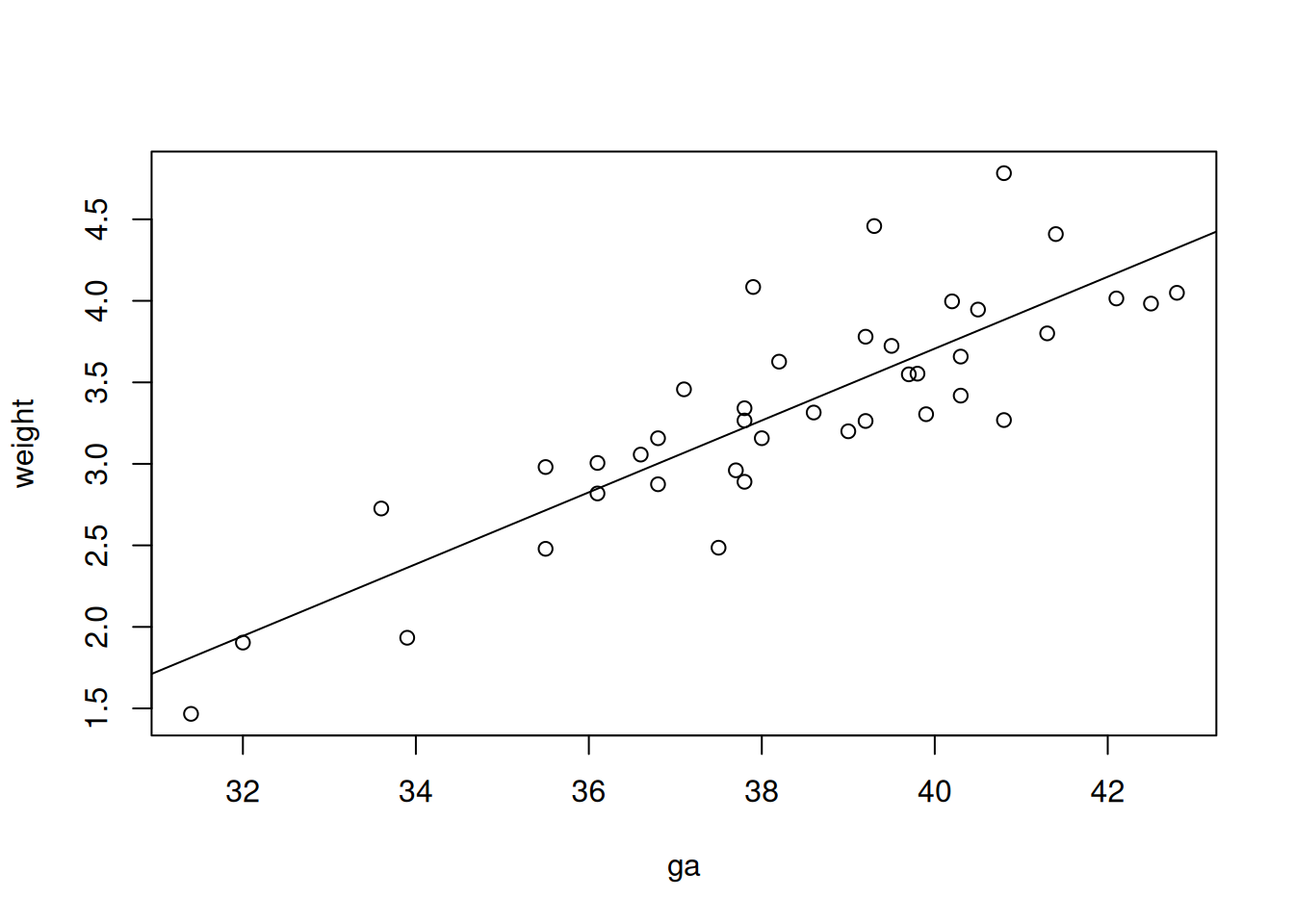
We can also plot the data with our fitted line overlaid:
5.6 Limitations of simple linear regression
Simple linear regression is useful, but it has important limitations:
- Only one covariate: Simple linear regression models the relationship between the response and a single covariate. In many real-world situations, multiple variables may influence the response.
- Linearity assumption: The model assumes that the relationship between the response and the covariate is linear. If the true relationship is non-linear, the model may not fit well.
- Constant variance (homoscedasticity): The errors are assumed to have constant variance across all values of the covariate. If the variance of the errors changes (heteroscedasticity), the model’s estimates and inferences may be unreliable.
- Normality of errors: The errors are assumed to be normally distributed. If this assumption is violated, inference based on the model may not be valid.
These limitations, and methods to address them, will be covered in more detail in the second-year module, Statistical Modelling I.