Chapter 4 Statistical Inference

4.1 Statistical modelling

4.1.1 Introduction

Statistical inference uses observed data to draw conclusions, make predictions, and support decisions. We do this by positing probability distributions (statistical models) for how the data are generated. For example, suppose the true proportion of mature students is $p$ with $0<p<1$. For a random sample of $n$ students, each observation can be modelled as Bernoulli($p$), taking value 1 for a mature student and 0 otherwise. Here the model is Bernoulli with success probability $p$.

To illustrate with another example, suppose we have observed fast food waiting times in the morning and afternoon, as in Example 1.1. If time is treated as continuous, each customer’s waiting time can be modelled as a normal random variable.

In general:

The model’s form helps us understand the data-generating process.
If a model explains the observed data well, it can inform predictions and decisions about future (unobserved) data.
Models, together with appropriate methodology, allow us to quantify uncertainty in conclusions, predictions, and decisions.

We use $x_1, x_2, \ldots, x_n$ for $n$ observations of random variables $X_1, $X_2, \ldots, X_n$ (uppercase for random variables, lowercase for observed values). For the fast food waiting time example, we have $n = 20$, $x_1 = 38, x_2 = 100, \ldots, x_{20} = 70$, and $X_i$ is the waiting time for the $i$th person in the sample.

4.1.2 Statistical models

Suppose we denote the complete data by the vector $\boldsymbol{x} = (x_1 , x_2 , \ldots , x_n)$ and use $\boldsymbol{X} = (X_1 , X_2 , \ldots , X_n)$ for the corresponding random variables. A statistical model specifies a probability distribution for the random variables $\boldsymbol{X}$ corresponding to the data observations $\boldsymbol{x}$. Providing a specification for the distribution of $n$ jointly varying random variables can be a daunting task, particularly if $n$ is large. However, this task is made much easier if we can make some simplifying assumptions, such as

$X_1 , X_2 , \ldots , X_n$ are independent random variables,
$X_1 , X_2 , \ldots , X_n$ have the same probability distribution (so $x_1 , x_2 , \ldots , x_n$ are observations of a single random variable $X$).

Assumption 1 depends on the sampling mechanism and is common in practice. For the Southampton student example, it requires random selection from all students. It is violated when samples are temporally or spatially correlated (e.g., daily air pollution over a year, or measurements from nearby locations). In this module we consider only data sets for which Assumption 1 is reasonable.

Assumption 2 is not always appropriate, but is often reasonable when modelling a single variable. In the fast food waiting time example, it requires no systematic AM–PM differences.

If Assumptions 1 and 2 both hold, then $X_1, \ldots, X_n$ are independent and identically distributed (i.i.d.).

4.1.3 A fully specified model

Sometimes a model fully specifies the distribution of $X_1, \ldots, X_n$. For example, $X \sim N(\mu,\sigma^2)$ with $\mu=100$ and $\sigma^2=100$ is fully specified: there are no unknowns to estimate (though we may still use data to assess plausibility). Such cases are uncommon unless external theory justifies the parameter values.

4.1.4 A parametric statistical model

A parametric statistical model specifies a family of distributions indexed by a finite set of parameters. The model’s form is fixed; only the parameter values are unknown. For example, the Poisson distribution is parameterised by the parameter $\lambda$ which happens to be the mean of the distribution; the normal distribution is parameterised by two parameters, the mean $\mu$ and the variance $\sigma^2$. When parameters are unknown (e.g., $\lambda$, $\mu$, $\sigma^2$), we estimate them from data. We discuss estimation next.

4.1.5 A nonparametric statistical model

Sometimes we avoid specifying a precise parametric form for the distribution of $X_1, \ldots, X_n$ (e.g., when a histogram is clearly non-normal). We may still assume $X_1, \ldots, X_n$ are i.i.d., but model them nonparametrically (distribution-free methods), without committing to a finite-dimensional parametric family.

Example 4.1 (Computer failures) Let $X$ denote the count of computer failures per week from Example 1.2, summarised in the following table:

0	1	2	3	4	5	6	7	8	9	10	11	12	13	17
12	16	21	12	11	8	7	2	4	2	3	2	2	1	1

We want to estimate how many weeks in the next year the system will fail at least once. The answer is $52 \times (1 - P(X=0))$. But how would you estimate $P (X = 0)$? Consider two approaches.

Nonparametric. Estimate $P (X = 0)$ by the relative frequency of number of zeros in the above sample, which is 12 out of 104. Thus our estimate of $P (X = 0)$ is $12/104$. Hence, our estimate of the number of weeks when there will be at least one computer failure is $52 \times (1 - 12/104) = 46$.
Parametric. Suppose we assume that $X$ follows the Poisson distribution with parameter $\lambda$. Then the answer to the above question is \[52 \times (1 - P (X = 0)) = 52 \times \left(1 - e^{-\lambda} \frac{\lambda^0}{0!} \right) = 52 \times (1 - e^{-\lambda})\] which involves the unknown parameter $\lambda$. For the Poisson distribution we know that $E(X) = \lambda$. Hence we could use the sample mean $\bar X$ to estimate $E(X) = \lambda$. Thus we estimate $\hat \lambda = \bar x = 3.75.$ This type of estimator is called a moment estimator. Now our estimate of the number of weeks when there will be at least one computer failure is $52 \times (1 - e^{-3.75}) = 50.78 \approx 51$, which is very different from our answer of 46 from the nonparametric approach.

4.1.6 Should we prefer parametric or nonparametric and why?

Prefer the parametric approach when its assumptions (e.g., Poisson for counts) are justified, assessed via plots or by comparing fitted probabilities \[\hat P(X=x)=e^{-\hat\lambda}\frac{\hat\lambda^x}{x!}\] to sample frequencies. Model-based analyses are often more precise and provide principled uncertainty quantification. Use nonparametric methods when the parametric model is not credible.

4.2 Estimation

4.2.1 Introduction

After collecting data and proposing a model, the first task is typically estimation.

For a parametric model, estimate the unknown parameters (e.g., for i.i.d. Poisson data, estimate $\lambda=E(X)$).
For a nonparametric model, estimate population features of $X$ (e.g., $\mu=E(X)$, $\sigma^2=\operatorname{Var}(X)$).

We use $\theta$ for the estimand (the quantity to be estimated). In the examples above, $\theta$ may be $\lambda$, or $\mu$, or $\sigma^2$.

4.2.2 Population and sample

Recall: a statistical model specifies a probability distribution for $\boldsymbol{X}$ corresponding to observations $\boldsymbol{x}$.

The observations $\boldsymbol{x} = (x_1 , \ldots , x_n )$ are called the sample, and quantities derived from the sample are sample quantities. For example, as in Chapter 1, we call \[\bar x = \frac{1}{n} \sum_{i=1}^n x_i\] the sample mean.
The probability distribution for $X$ specified in our model represents all possible observations which might have been observed in our sample, and is therefore sometimes referred to as the population. Quantities derived from this distribution are population quantities. For example, if our model is that $X_1 , \ldots , X_n$ are i.i.d., following the common distribution of a random variable $X$, then we call $E(X)$ the population mean.

4.2.3 Statistic and estimator

A statistic $T(\boldsymbol{x})$ is any function of the observed data $x_{1}, \ldots, x_{n}$ (and does not depend on unknowns). An estimate of $\theta$ is a statistic used to estimate $\theta$, denoted $\tilde{\theta}(\boldsymbol{x})$. The corresponding random variable $\tilde{\theta}(\boldsymbol{X})$ is the estimator. An estimate is a realised number (e.g., $\bar{x}$); an estimator is a random variable (e.g., $\bar{X}$).

The probability distribution of $\tilde{\theta}(\boldsymbol{X})$ is its sampling distribution. The estimate $\tilde{\theta}(\boldsymbol{x})$ is one realisation from that distribution.

Example 4.2 Suppose that we have a random sample $X_{1}, \ldots, X_{n}$ from the uniform distribution on the interval $(0, \theta)$ where $\theta>0$ is unknown. Suppose that $n=5$ and we have the sample observations $x_{1}=2.3, x_{2}=3.6, x_{3}=20.2, x_{4}=0.9, x_{5}=17.2$. We aim to estimate $\theta$. How can we proceed?

Here the pdf $f(x)=\frac{1}{\theta}$ for $0 \leq x \leq \theta$ and 0 otherwise. Hence $E(X)=\int_{0}^{\theta} \frac{1}{\theta} x d x=\frac{\theta}{2}$. There are many possible estimators for $\theta$, e.g. $\hat{\theta}_{1}(\boldsymbol{X})=2 \bar{X}$, which is motivated by the method of moments because $\theta=2 E(X)$. A second estimator is $\hat{\theta}_{2}(\boldsymbol{X})=\max \left\{X_{1}, X_{2}, \ldots, X_{n}\right\}$, which is intuitive since $\theta$ must be greater than or equal to all observed values and thus the maximum of the sample value will be closest to $\theta$.

How should we choose between $\hat{\theta}_{1}$ and $\hat{\theta}_{2}$? We need the sampling distributions to assess bias and variability (defined next). First, derive the distribution of $\hat{\theta}_{2}$. Let $Y=\hat{\theta}_{2}(\boldsymbol{X})=\max\{X_{1},\ldots,X_{n}\}$. For $0<y<\theta$, the cdf is \[\begin{align*} P(Y \leq y) &=P\left(\max \left\{X_{1}, X_{2}, \ldots, X_{n}\right\} \leq y\right) \\ &\left.=P\left(X_{1} \leq y, X_{2} \leq y, \ldots, X_{n} \leq y\right)\right) \quad \text{since max $\leq y$ if and only if each $\leq y$}] \\ &=P\left(X_{1} \leq y\right) P\left(X_{2} \leq y\right) \cdots P\left(X_{n} \leq y\right) \quad \text {since the $X_i$ are independent}\\ &=\frac{y}{\theta} \times \frac{y}{\theta} \times \cdots \times \frac{y}{\theta} \\ &=\left(\frac{y}{\theta}\right)^{n} . \end{align*}\]

Now the pdf of $Y$ is \[f(y)=\frac{d F(y)}{d y}=n \frac{y^{n-1}}{\theta^{n}}, \quad 0 \leq y \leq \theta.\] Using this pdf, it can be shown that $E\left(\hat{\theta}_{2}\right)=E(Y)=\frac{n}{n+1} \theta,$ and \[\operatorname{Var}\left(\hat{\theta}_{2}\right)=\frac{n \theta^{2}}{(n+2)(n+1)^{2}}.\]

4.2.4 Bias and mean square error

In the uniform distribution example we saw that the estimator $\hat{\theta}_{2}=Y=\max \left\{X_{1}, X_{2}, \ldots, X_{n}\right\}$ is a random variable and its pdf is given by $f(y)=n \frac{y^{n-1}}{\theta^{n}}$ for $0 \leq y \leq \theta$. This probability distribution is called the sampling distribution of $\hat{\theta}_{2}$. From this we have seen that $E\left(\hat{\theta}_{2}\right)=\frac{n}{n+1} \theta$.

In general, we define the bias of an estimator $\tilde{\theta}(\boldsymbol{X})$ of $\theta$ to be \[\operatorname{bias}(\tilde{\theta})=E(\tilde{\theta})-\theta.\]

An estimator $\tilde{\theta}(\boldsymbol{X})$ is said to be unbiased if \[\operatorname{bias}(\tilde{\theta})=0 \text {, i.e. if } E(\tilde{\theta})=\theta.\]

Thus an estimator is unbiased if its expected value equals the target: “right on average” under repeated sampling.

Thus for the uniform distribution example, $\hat{\theta}_{2}$ is a biased estimator of $\theta$ and \[\operatorname{bias}\left(\hat{\theta}_{2}\right)=E\left(\hat{\theta}_{2}\right)-\theta=\frac{n}{n+1} \theta-\theta=-\frac{1}{n+1} \theta,\] which goes to zero as $n \rightarrow \infty$. However, $\hat{\theta}_{1}=2 \bar{X}$ is unbiased since $E\left(\hat{\theta}_{1}\right)=2 E(\bar{X})=2 \frac{\theta}{2}=\theta$.

Unbiasedness does not guarantee estimates close to $\theta$. A more informative measure is the mean squared error (MSE), defined as \[\operatorname{MSE}(\tilde{\theta})=E\left[(\tilde{\theta}-\theta)^{2}\right]\]

If $\tilde{\theta}$ is unbiased ($E(\tilde{\theta})=\theta$), then $\operatorname{MSE}(\tilde{\theta})=\operatorname{Var}(\tilde{\theta})$. In general:

Theorem 4.1 \[\operatorname{MSE}(\tilde{\theta})=\operatorname{Var}(\tilde{\theta})+\operatorname{bias}(\tilde{\theta})^{2}\]

The proof is similar to the proof of Theorem 1.1.

Proof. \[\begin{align*} \operatorname{MSE}(\tilde{\theta}) &=E\left[(\tilde{\theta}-\theta)^{2}\right] \\ &=E\left[(\tilde{\theta}-E(\tilde{\theta})+E(\tilde{\theta})-\theta)^{2}\right] \\ &=E\left[(\tilde{\theta}-E(\tilde{\theta}))^{2}+(E(\tilde{\theta})-\theta)^{2}+2(\tilde{\theta}-E(\tilde{\theta}))(E(\tilde{\theta})-\theta)\right] \\ &=E[\tilde{\theta}-E(\tilde{\theta})]^{2}+E[E(\tilde{\theta})-\theta]^{2}+2 E[(\tilde{\theta}-E(\tilde{\theta}))(E(\tilde{\theta})-\theta)] \\ &=\operatorname{Var}(\tilde{\theta})+[E(\tilde{\theta})-\theta]^{2}+2(E(\tilde{\theta})-\theta) E[(\tilde{\theta}-E(\tilde{\theta}))] \\ &=\operatorname{Var}(\tilde{\theta})+\operatorname{bias}(\tilde{\theta})^{2}+2(E(\tilde{\theta})-\theta)[E(\tilde{\theta})-E(\tilde{\theta})] \\ &=\operatorname{Var}(\tilde{\theta})+\operatorname{bias}(\tilde{\theta})^{2} . \end{align*}\]

Example 4.3 Continuing the $U(0,\theta)$ example: $\hat{\theta}_{1}=2\bar{X}$ is unbiased, whereas $\operatorname{bias}(\hat{\theta}_{2})=-\frac{1}{n+1}\theta$. How do they compare via MSE? Since $\hat{\theta}_{1}$ is unbiased, its MSE equals its variance. Later we prove that for a random sample from any population \[\operatorname{Var}(\bar{X})=\frac{\operatorname{Var}(X)}{n},\] where $\operatorname{Var}(X)$ is the variance of the population sampled from. Returning to our example, we know that if $X \sim U(0, \theta)$ then $\operatorname{Var}(X)=\frac{\theta^{2}}{12}$. Therefore we have \[ \operatorname{MSE}\left(\hat{\theta}_{1}\right)=\operatorname{Var}\left(\hat{\theta}_{1}\right)=\operatorname{Var}(2 \bar{X})=4 \operatorname{Var}(\bar{X})=4 \frac{\theta^{2}}{12 n}=\frac{\theta^{2}}{3 n} . \]

Now, for $\hat{\theta}_{2}$ we know that:

$\operatorname{Var}\left(\hat{\theta}_{2}\right)=\frac{n \theta^{2}}{(n+2)(n+1)^{2}}$
$\operatorname{bias}\left(\hat{\theta}_{2}\right)=-\frac{1}{n+1} \theta$.

Now \[\begin{align*} \operatorname{MSE}\left(\hat{\theta}_{2}\right) &=\operatorname{Var}\left(\hat{\theta}_{2}\right)+\operatorname{bias}\left(\hat{\theta}_{2}\right)^{2} \\ &=\frac{n \theta^{2}}{(n+2)(n+1)^{2}}+\frac{\theta^{2}}{(n+1)^{2}} \\ &=\frac{\theta^{2}}{(n+1)^{2}}\left(\frac{n}{n+2}+1\right) \\ &=\frac{\theta^{2}}{(n+1)^{2}} \frac{2 n+2}{n+2} . \end{align*}\] The MSE of $\hat{\theta}_{2}$ is an order of magnitude smaller than the MSE of $\hat{\theta}_{1}$ (of order $1/n^{2}$ rather than $1/n$), providing justification for the preference of $\hat{\theta}_{2}=\max \left\{X_{1}, X_{2}, \ldots, X_{n}\right\}$ as an estimator of $\theta$.

4.3 Estimating the population mean

4.3.1 Introduction

A common task is to estimate a population mean, together with its uncertainty. Point estimates without uncertainty are often uninformative. For example, “ice-free within 20–30 years” conveys both a central value and a range. Here we introduce the standard error of an estimator to quantify uncertainty in estimating a population mean.

4.3.2 Estimation of a population mean

Suppose that $X_{1}, \ldots, X_{n}$ is a random sample from any probability distribution $f(x)$, which may be discrete or continuous. Suppose that we want to estimate the unknown population mean $E(X)=\mu$ and variance, $\operatorname{Var}(X)=\sigma^{2}$. In order to do this, it is not necessary to make any assumptions about $f(x)$, so this may be thought of as nonparametric inference.

We have the following results:

Theorem 4.2 Suppose $X_1, \ldots, X_n$ is a random sample, with $E(X)=\mu$. The sample mean \[\bar{X}=\frac{1}{n} \sum_{i=1}^{n} X_{i}\] is an unbiased estimator of $\mu=E(X)$, i.e. $E(\bar{X})=\mu$.

In other words, the sample mean is an unbiased estimator of the population mean.

Proof. We have \[E[\bar{X}]=\frac{1}{n} \sum_{i=1}^{n} E\left(X_{i}\right)=\frac{1}{n} \sum_{i=1}^{n} E(X)=E(X)\] so $\bar{X}$ is an unbiased estimator of $E(X)$.

Theorem 4.3 Suppose $X_1, \ldots, X_n$ is a random sample, with $\operatorname{Var}(X)=\sigma^{2}$. Then \[\operatorname{Var}(\bar{X})=\frac{\sigma^{2}}{n}.\]

Proof. Using that for independent variables the variance of a sum equals the sum of variances (Section 3.7), we have \[\operatorname{Var}[\bar{X}]=\frac{1}{n^{2}} \sum_{i=1}^{n} \operatorname{Var}\left(X_{i}\right)=\frac{1}{n^{2}} \sum_{i=1}^{n} \operatorname{Var}(X)=\frac{n}{n^{2}} \operatorname{Var}(X)=\frac{\sigma^{2}}{n},\]

Together, Theorems 4.2 and 4.3 imply that the MSE of $\bar{X}$ is $\operatorname{Var}(X) / n$.

Theorem 4.4 Suppose $X_1, \ldots, X_n$ is a random sample, with $\operatorname{Var}(X)=\sigma^{2}$. The sample variance with divisor $n-1$ \[S^{2}=\frac{1}{n-1} \sum_{i=1}^{n}\left(X_{i}-\bar{X}\right)^{2}\] is an unbiased estimator of $\sigma^{2}$, i.e. $E\left(S^{2}\right)=\sigma^{2}$.

In other words, the sample variance is an unbiased estimator of the population variance.

Proof. We need to show $E\left(S^{2}\right)=\sigma^{2}$. We have \[S^{2}=\frac{1}{n-1} \sum_{i=1}^{n}\left(X_{i}-\bar{X}\right)^{2}=\frac{1}{n-1}\left[\sum_{i=1}^{n} X_{i}^{2}-n \bar{X}^{2}\right].\] To evaluate the expectation of the above, we need $E\left(X_{i}^{2}\right)$ and $E\left(\bar{X}^{2}\right)$. In general, we know for any random variable, \[\operatorname{Var}(Y)=E\left(Y^{2}\right)-(E(Y))^{2} \quad \Rightarrow E\left(Y^{2}\right)=\operatorname{Var}(Y)+(E(Y))^{2}.\] Thus, we have \[E\left(X_{i}^{2}\right)=\operatorname{Var}\left(X_{i}\right)+\left(E\left(X_{i}\right)\right)^{2}=\sigma^{2}+\mu^{2},\] and \[E\left(\bar{X}^{2}\right)=\operatorname{Var}(\bar{X})+(E(\bar{X}))^{2}=\sigma^{2} / n+\mu^{2},\] from Theorems 4.2 and 4.3. So \[\begin{align*} E\left(S^{2}\right) &=E\left\{\frac{1}{n-1}\left[\sum_{i=1}^{n} X_{i}^{2}-n \bar{X}^{2}\right]\right\} \\ &=\frac{1}{n-1}\left[\sum_{i=1}^{n} E\left(X_{i}^{2}\right)-n E\left(\bar{X}^{2}\right)\right] \\ &=\frac{1}{n-1}\left[\sum_{i=1}^{n}\left(\sigma^{2}+\mu^{2}\right)-n\left(\sigma^{2} / n+\mu^{2}\right)\right] \\ &=\frac{1}{n-1}\left[n \sigma^{2}+n \mu^{2}-\sigma^{2}-n \mu^{2}\right] \\ &=\sigma^{2} \equiv \operatorname{Var}(X) . \end{align*}\]

4.3.3 Standard deviation and standard error

For an unbiased estimator $\tilde{\theta}$, \[\operatorname{MSE}(\tilde{\theta})=\operatorname{Var}(\tilde{\theta})\] and therefore the sampling variance of the estimator is an important summary of its quality.

We usually prefer to focus on the standard deviation of the sampling distribution of $\tilde{\theta}$, \[\text {s.d.}(\tilde{\theta})=\sqrt{\operatorname{Var}(\tilde{\theta})}.\]

In practice s.d.$(\tilde{\theta})$ is unknown, but we can estimate it from the sample. The standard error, s.e.$(\tilde{\theta})$, is an estimate of the standard deviation of the sampling distribution of $\tilde{\theta}$.

We proved that \[\operatorname{Var}[\bar{X}]=\frac{\sigma^{2}}{n} \Rightarrow \text { s.d. }(\bar{X})=\frac{\sigma}{\sqrt{n}}.\]

As $\sigma$ is unknown, we cannot calculate this standard deviation. However, we know that $E\left(S^{2}\right)=\sigma^{2}$, i.e. that the sample variance is an unbiased estimator of the population variance. Hence $S^{2} / n$ is an unbiased estimator for $\operatorname{Var}(\bar{X})$. Therefore we obtain the standard error of the mean, s.e. $(\bar{X})$, by plugging in the estimate \[s=\left(\frac{1}{n-1} \sum_{i=1}^{n}\left(x_{i}-\bar{x}\right)^{2}\right)^{1 / 2}\] of $\sigma$ into s.d.$(\bar{X})$ to obtain \[\text {s.e.}(\bar{X})=\frac{s}{\sqrt{n}}.\]

For the computer failure data, the estimate $\bar{x}=3.75$ has standard error \[\text{s.e.}(\bar{X})=\frac{3.381}{\sqrt{104}}=0.332.\]

This is one choice of standard error. Under parametric assumptions about $f(x)$, alternative (often smaller) standard errors may be available. For example, if $X_{1}, \ldots, X_{n}$ are i.i.d. $\operatorname{Poisson}(\lambda)$ random variables, $E(X)=\lambda$, so $\bar{X}$ is an unbiased estimator of $\lambda$. $\operatorname{Var}(X)=\lambda$, so another $\text{s.e.}(\bar{X})=\sqrt{\hat{\lambda} / n}=\sqrt{\bar{x} / n}$. In the computer failure data example, this is $\sqrt{\frac{3.75}{104}}=0.19$.

4.4 Confidence intervals

4.4.1 Introduction

An estimate $\tilde{\theta}$ of a parameter $\theta$ is sometimes referred to as a point estimate. The usefulness of a point estimate is enhanced if some kind of measure of its precision can also be provided. Usually, for an unbiased estimator, this will be a standard error, an estimate of the standard deviation of the associated estimator, as we have discussed previously. An alternative summary of the information provided by the observed data about the location of a parameter $\theta$ and the associated precision is a confidence interval.

Suppose that $x_{1}, \ldots, x_{n}$ are observations of random variables $X_{1}, \ldots, X_{n}$ whose joint pdf is specified apart from a single parameter $\theta$. To construct a confidence interval for $\theta$, we need to find a random variable $T(\mathbf{X}, \theta)$ whose distribution does not depend on $\theta$ and is therefore known. This random variable $T(\mathbf{X}, \theta)$ is called a pivot for $\theta$. Hence we can find numbers $h_{1}$ and $h_{2}$ such that \[\begin{equation} P\left(h_{1} \leq T(\mathbf{X}, \theta) \leq h_{2}\right)=1-\alpha \tag{4.1} \end{equation}\] where $1-\alpha$ is any specified probability. If (4.1) can be ‘inverted’,we can write it as \[P\left(g_{1}(\mathbf{X}) \leq \theta \leq g_{2}(\mathbf{X})\right)=1-\alpha.\]

Thus, with probability $1-\alpha$, the random interval $(g_{1}(\mathbf{X}), g_{2}(\mathbf{X}))$ contains $\theta$. After observing $x_{1}, \ldots, x_{n}$ we obtain the realised interval $(g_{1}(\mathbf{x}), g_{2}(\mathbf{x}))$, a $100(1-\alpha)\%$ confidence interval for $\theta$. Over repeated samples, $100(1-\alpha)\%$ of such intervals would contain $\theta$. Common levels are 90%, 95%, and 99%.

4.4.2 Confidence interval for a normal mean

Let $X_{1}, \ldots, X_{n}$ be i.i.d. $N\left(\mu, \sigma^{2}\right)$ random variables. From the Central Limit Theorem (Section 3.8), we know that for large $n$, \[\bar{X} \sim N\left(\mu, \sigma^{2} / n\right) \quad \Rightarrow \quad \sqrt{n} \frac{(\bar{X}-\mu)}{\sigma} \sim N(0,1).\]

Suppose we know that $\sigma=10$, so $\sqrt{n}(\bar{X}-\mu) / \sigma$ is a pivot for $\mu$. Then we can use the distribution function of the standard normal distribution to find values $h_{1}$ and $h_{2}$ such that \[P\left(h_{1} \leq \sqrt{n} \frac{(\bar{X}-\mu)}{\sigma} \leq h_{2}\right)=1-\alpha\] for a chosen value of $1-\alpha$ which is called the confidence level. So $h_{1}$ and $h_{2}$ are chosen so that the shaded area in Figure 4.1 is equal to the confidence level $1-\alpha$.

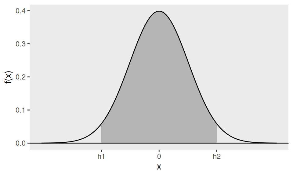
$h_1$ and $h_2$ are chosen to make the shaded area equal to the confidence level $1-\alpha$

Figure 4.1: $h_1$ and $h_2$ are chosen to make the shaded area equal to the confidence level $1-\alpha$

It is common to choose a symmetric interval, allocating $\alpha/2$ to each tail, so \[-h_{1}=h_{2} \equiv h \quad \text { and } \quad \Phi(h)=1-\frac{\alpha}{2}.\]

The most common choice of confidence level is $1-\alpha=0.95$, in which case $h=1.96=\texttt{qnorm(0.975)}$. You may also occasionally see $90\%$ ($h=1.645=\texttt{qnorm(0.95)}$) or $99\%$ ($h=2.58=\texttt{qnorm(0.995)}$) intervals.

Therefore we have \[\begin{align*} & P\left(-1.96 \leq \sqrt{n} \frac{(\bar{X}-\mu)}{\sigma} \leq 1.96\right)=0.95 \\ \Rightarrow & P\left(\bar{X}-1.96 \frac{\sigma}{\sqrt{n}} \leq \mu \leq \bar{X}+1.96 \frac{\sigma}{\sqrt{n}}\right)=0.95 . \end{align*}\]

Hence, $\bar{X}-1.96 \frac{\sigma}{\sqrt{n}}$ and $\bar{X}+1.96 \frac{\sigma}{\sqrt{n}}$ are the endpoints of a random interval which includes $\mu$ with probability $0.95$. The observed value of this interval, $\left(\bar{x} \pm 1.96 \frac{\sigma}{\sqrt{n}}\right)$, is called a 95% confidence interval for $\mu$.

Example 4.4 (Fast food waiting times) For the fast food waiting time data, we have $n=20$ data points combined from the morning and afternoon data sets. We have $\bar{x}=67.85$ and $n=20$. Hence, under the normal model assuming (just for the sake of illustration) $\sigma=18$, a 95% confidence interval for $\mu$ is

\[\begin{gathered} 67.85-1.96(18 / \sqrt{20}) \leq \mu \leq 67.85+1.96(18 / \sqrt{20}) \\ \Rightarrow 59.96 \leq \mu \leq 75.74 \end{gathered}\]

The R command is

mean(fastfood) + c(-1, 1) * qnorm(0.975) * 18 / sqrt (20)

assuming fastfood is the vector containing 20 waiting times.

In practice $\sigma$ is usually unknown, so we use alternative methods (next sections).

4.4.3 Some remarks about confidence intervals

Notice that $\bar{x}$ is an unbiased estimate of $\mu, \sigma / \sqrt{n}$ is the standard error of the estimate and $1.96$ (in general $h$ in the above discussion) is a critical value from the associated known sampling distribution. The formula $(\bar{x} \pm 1.96 \sigma / \sqrt{n})$ for the confidence interval is then generalised as: \[\text { Estimate } \pm \text { Critical value } \times \text { Standard error }\] where the estimate is $\bar{x}$, the critical value is $1.96$ and the standard error is $\sigma / \sqrt{n}$. We will see that this formula holds in many examples, but not all.
A $100(1-\alpha)\%$ confidence interval is one realisation from a procedure that contains $\theta$ in $100(1-\alpha)\%$ of repeated samples.
A confidence interval is not a probability statement about $\theta$ (a fixed constant in classical inference). Avoid statements like $P(1.3<\theta<2.2)=0.95$.
Misinterpreting CIs as probability intervals can mislead. For example, if $X_1,X_2 \sim U(\theta-1/2,\theta+1/2)$ i.i.d., then $(\min(x_1,x_2), \max(x_1,x_2))$ is a 50% CI for $\theta$, but after observing $(0.3,0.9)$ it is not correct to assert $P(0.3<\theta<0.9)=0.5$.

4.4.4 Confidence intervals using the CLT

4.4.4.1 Introduction

Confidence intervals are generally difficult to find. The difficulty lies in finding a pivot, i.e. a statistic $T(\mathbf{X}, \theta)$ such that \[P\left(h_{1} \leq T(\mathbf{X}, \theta) \leq h_{2}\right)=1-\alpha\] for two suitable numbers $h_{1}$ and $h_{2}$, and also that the above can be inverted to put the unknown $\theta$ in the middle of the inequality inside the probability statement. One approach is to use the Central Limit Theorem (CLT) to approximate normality and follow the normal-mean construction, replacing the unknown s.d. by its estimate.

4.4.4.2 Confidence intervals for $\mu$ using the CLT

The CLT allows us to assume the large sample approximation \[\sqrt{n} \frac{(\bar{X}-\mu)}{\sigma} \stackrel{\text { approx }}{\sim} N(0,1) \text { as } n \rightarrow \infty.\] Thus an approximate 95% CI for $\mu$ is $\bar{x} \pm 1.96\, \sigma/\sqrt{n}$. Since $\sigma$ is unknown, we replace it with an estimate (the s.e.), giving the familiar form: \[\text { Estimate } \pm \text { Critical value } \times \text { Standard error }\]

Suppose that we do not assume any distribution for the sampled random variable $X$ but assume only that $X_{1}, \ldots, X_{n}$ are i.i.d, following the distribution of $X$ where $E(X)=\mu$ and $\operatorname{Var}(X)=\sigma^{2}$. We know that the standard error of $\bar{X}$ is $s / \sqrt{n}$ where $s$ is the sample standard deviation with divisor $n-1$. Then the following provides an (approximate) $95 \%$ CI for $\mu$: \[\bar{x} \pm 1.96 \frac{s}{\sqrt{n}}.\]

Example 4.5 (Computer failures) For the computer failure data, $\bar{x}=3.75, s=3.381$ and $n=104$. Under the model that the data are observations of i.i.d. random variables with population mean $\mu$ (but no other assumptions about the underlying distribution), we compute a 95% confidence interval for $\mu$ to be \[\left(3.75-1.96 \frac{3.381}{\sqrt{104}}, 3.75+1.96 \frac{3.381}{\sqrt{104}}\right)=(3.10,4.40).\]

If we can assume a distribution for $X$, i.e. a parametric model for $X$, then we can do slightly better in estimating the standard error of $\bar{X}$ and as a result we can improve upon the previously obtained $95 \%$ CI. Two examples follow.

Example 4.6 (Poisson) If $X_{1}, \ldots, X_{n}$ are modelled as i.i.d. Poisson $(\lambda)$ random variables, then $\mu=\lambda$ and $\sigma^{2}=\lambda$. We know $\operatorname{Var}(\bar{X})=\sigma^{2} / n=\lambda / n$. Hence a standard error is $\sqrt{\hat{\lambda} / n}=\sqrt{\bar{x} / n}$ since $\hat{\lambda}=\bar{X}$ is an unbiased estimator of $\lambda$. Thus a 95% CI for $\mu=\lambda$ is given by \[\bar{x} \pm 1.96 \sqrt{\frac{\bar{x}}{n}}.\]

For the computer failure data, $\bar{x}=3.75, s=3.381$ and $n=104$. Under the model that the data are observations of i.i.d. random variables following a Poisson distribution with population mean $\lambda$, we compute a $95 \%$ confidence interval for $\lambda$ as \[\bar{x} \pm 1.96 \sqrt{\frac{\bar{x}}{n}}=3.75 \pm 1.96 \sqrt{3.75 / 104}=(3.38,4.12).\]

We see that this interval is narrower $(0.74=4.12-3.38)$ than the earlier interval $(3.10,4.40)$, which has a length of $1.3$. We prefer narrower confidence intervals as they facilitate more accurate inference regarding the unknown parameter.

Example 4.7 (Bernoulli) If $X_{1}, \ldots, X_{n}$ are modelled as i.i.d. Bernoulli $(p)$ random variables, then $\mu=p$ and $\sigma^{2}=p(1-p)$. We know $\operatorname{Var}(\bar{X})=\sigma^{2} / n=p(1-p) / n$. Hence a standard error is $\sqrt{\hat{p}(1-\hat{p}) / n}=\sqrt{\bar{x}(1-\bar{x}) / n}$, since $\hat{p}=\bar{X}$ is an unbiased estimator of $p$. Thus a $95 \%$ CI for $\mu=p$ is given by \[\bar{x} \pm 1.96 \sqrt{\frac{\bar{x}(1-\bar{x})}{n}}.\]

For the example, suppose $\bar{x}=0.2$ and $n=10$. Then we obtain the $95 \%$ CI as \[0.2 \pm 1.96 \sqrt{(0.2 \times 0.8) / 10}=(-0.048,0.448)\]

Here $n$ is too small for the large-sample approximation to be accurate.

4.4.5 Exact confidence interval for the normal mean

For normal models we do not have to rely on large sample approximations, because it turns out that the distribution of \[T=\frac{\sqrt{n}(\bar{X}-\mu)}{S},\] where $S^{2}$ is the sample variance with divisor $n-1$, is standard (easily calculated) and thus the statistic $T=T(\mathbf{X}, \mu)$ can be an exact pivot for any sample size $n>1$.

For any chosen $1-\alpha$ (e.g., 0.95) we can find $h$ such that $P(-h<T<h)=1-\alpha$. Note that $T$ does not involve the unknown variance $\sigma^{2}$. Proceed as follows to obtain the exact CI for $\mu$: \[\begin{align*} & P(-h \leq T \leq h)=1-\alpha \\ \text { i.e. } & P\left(-h \leq \sqrt{n} \frac{(\bar{X}-\mu)}{S} \leq h\right)=0.95 \\ \Rightarrow & P\left(\bar{X}-h \frac{S}{\sqrt{n}} \leq \mu \leq \bar{X}+h \frac{S}{\sqrt{n}}\right)=0.95 \end{align*}\]

The observed value of this interval, $\left(\bar{x} \pm h \frac{s}{\sqrt{n}}\right)$, is the $95 \%$ confidence interval for $\mu$. Remarkably, this also of the general form, \[\text { Estimate } \pm \text { Critical value } \times \text { Standard error },\] where the critical value is $h$ and the standard error of the sample mean is $\frac{s}{\sqrt{n}}$. Now, how do we find the critical value $h$ for a given $1-\alpha$ ? We need to introduce the $t$-distribution.

Let $X_{1}, \ldots, X_{n}$ be i.i.d $N\left(\mu, \sigma^{2}\right)$ random variables. Define $\bar{X}=\frac{1}{n} \sum_{i=1}^{n} X_{i}$ and \[S^{2}=\frac{1}{n-1}\left(\sum_{i=1}^{n} X_{i}^{2}-n \bar{X}^{2}\right).\] Then, it can be shown (see Statistical Inference in second year) that \[\sqrt{n} \frac{(\bar{X}-\mu)}{S} \sim t_{n-1},\] where $t_{n-1}$ denotes the standard $t$ distribution with $n-1$ degrees of freedom. The standard $t$ distribution is a family of distributions which depend on one parameter called the degrees-of-freedom (df) which is $n-1$ here. The concept of degrees of freedom is that it is usually the number of independent random samples, $n$ here, minus the number of linear parameters estimated, 1 here for $\mu$. Hence the df is $n-1$.

The probability density function of the $t_{k}$ distribution is similar to a standard normal, in that it is symmetric around zero and ‘bell-shaped’, but the t-distribution is more heavy-tailed, giving greater probability to observations further away from zero. Figure 4.2 illustrates the $t_{k}$ density function for various values of $k$.

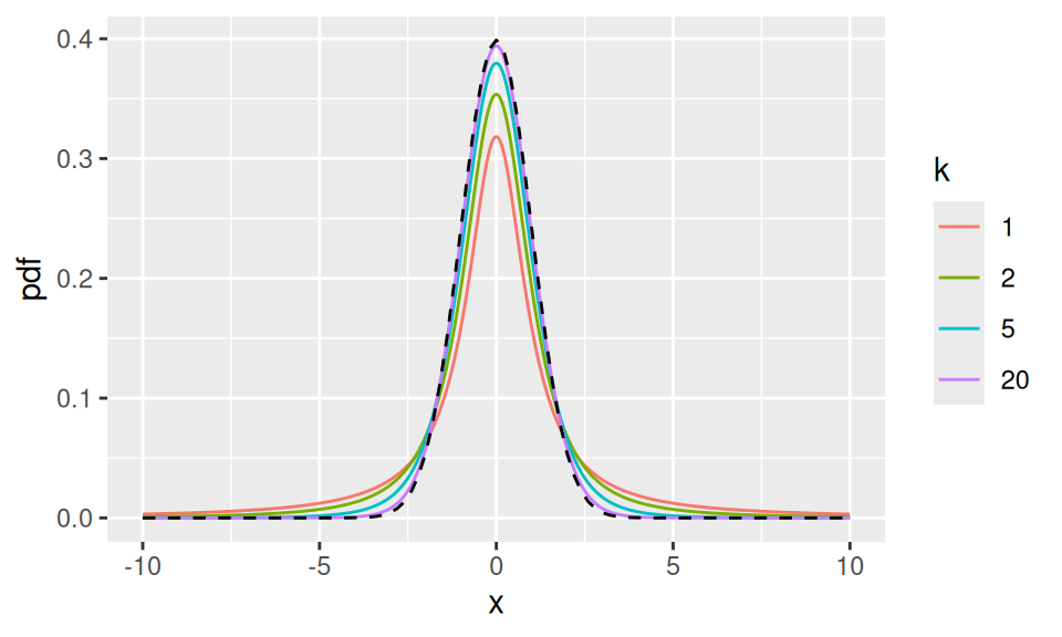
Figure 4.2: The pdf of the $t_k$ distribution for various values of $k$. The dashed line is the standard normal pdf.

The values of $h$ for a given $1-\alpha$ can be obtained using the R command (abbreviation for quantile of $t$ ). For example, we can find $h$ for $1-\alpha=0.95$ and $n=20$

qt(0.975, df = 19)

## [1] 2.093024

Note that it should be $0.975$ so that we are splitting $0.05$ probability between the two tails equally and the df should be $n-1=19$. Indeed, modifying the above command, we obtain the following critical values for the $95 \%$ interval for different values of the sample size $n$.

As $n \to \infty$, $h$ approaches 1.96 (the normal critical value), since $t_{n-1}$ converges to the standard normal.

If you can justify that the underlying distribution is normal then you can use the $t$-distribution-based confidence interval.

Example 4.8 (Fast food waiting times) We would like to find a confidence interval for the true mean waiting time. If $X$ denotes the waiting time in seconds, we have $n=20, \bar{x}=67.85$, $s=18.36$. Hence, recalling that the critical value $h=2.093$, from the command , a $95 \%$ confidence interval for $\mu$ is \[\begin{align*} 67.85-2.093 \times 18.36 / \sqrt{20} \leq \mu & \leq 67.85+2.093 \times 18.36 / \sqrt{20} \\ \Rightarrow 59.26 & \leq \mu \leq 76.44 . \end{align*}\]

In R, if the vector fastfood contains all the service times, we can find a $95 \%$ confidence interval with

mean(fastfood) + c(-1, 1) * qt(0.975, df = 19) * sd(fastfood) / sqrt(20)

## [1] 59.25467 76.44533

or a $90 \%$ confidence interval with

mean(fastfood) + c(-1, 1) * qt(0.95, df = 19) * sd(fastfood) / sqrt(20)

## [1] 60.74905 74.95095

or a $99 \%$ confidence interval with

mean(fastfood) + c(-1, 1) * qt(0.995, df = 19) * sd(fastfood) / sqrt(20)

## [1] 56.10113 79.59887

We see that the interval widens as the confidence level increases.

Example 4.9 (Weight gain) Returning to the weight gain data from Example 1.3, we would like to find a confidence interval for the true average weight gain (final weight - initial weight). Here $n=68, \bar{x}=0.8672$ and $s=0.9653$. Hence, a $95 \%$ confidence interval for $\mu$ is \[\begin{align*} 0.8672-1.996 \times 0.9653 / \sqrt{68} \leq \mu & \leq 0.8672+1.996 \times 0.9653 / \sqrt{68} \\ \Rightarrow 0.6335 & \leq \mu \leq 1.1008 \end{align*}\]

In R, we obtain the critical value $1.996$ by

qt(0.975, df = 67)

## [1] 1.996008

Note that the interval here does not include the value 0, so it is very likely that the weight gain is significantly positive, which we will justify using what is called hypothesis testing.

4.5 Hypothesis testing

4.5.1 Hypothesis testing in general

4.5.1.1 Introduction

Managers and researchers often make claims (e.g., average waiting time < 1 minute; phones never fail in three years; students gain weight in their first year away from home). How can we assess such claims? We use hypothesis testing.

In statistical inference, we use observations $x_{1}, \ldots, x_{n}$ of univariate random variables $X_{1}, \ldots, X_{n}$ in order to draw inferences about the probability distribution $f(x)$ of the underlying random variable $X$. So far, we have mainly been concerned with estimating features (usually unknown parameters) of $f(x)$. It is often of interest to compare alternative specifications for $f(x)$. If we have a set of competing probability models which might have generated the observed data, we may want to determine which of the models is most appropriate. A proposed (hypothesised) model for $X_{1}, \ldots, X_{n}$ is then referred to as a hypothesis, and pairs of models are compared using hypothesis tests.

For example, let $H_0$ and $H_1$ specify competing distributions $f^{(0)}(x)$ and $f^{(1)}(x)$ that fully determine the joint distribution of $X_{1},\ldots,X_{n}$; these are simple hypotheses. Often both take the same parametric form $f(x;\theta)$ with different specified values $\theta^{(0)} \neq \theta^{(1)}$.

More generally, hypotheses may leave parameters unspecified (composite hypotheses). For instance, $X_{1},\ldots,X_{n}$ i.i.d. from $f(x;\theta)$ with $\theta<0$ does not fully specify probabilities without a particular $\theta$.

Examples of hypotheses:

$X_{1}, \ldots, X_{n} \sim N\left(\mu, \sigma^{2}\right)$ with $\mu=0, \sigma^{2}=2$.
$X_{1}, \ldots, X_{n} \sim N\left(\mu, \sigma^{2}\right)$ with $\mu=0, \sigma^{2} \in \mathcal{R}_{+}$.
$X_{1}, \ldots, X_{n} \sim N\left(\mu, \sigma^{2}\right)$ with $\mu \neq 0, \sigma^{2} \in \mathcal{R}_{+}$.
$X_{1}, \ldots, X_{n} \sim \operatorname{Bernoulli}(p)$ with $p=\frac{1}{2}$.
$X_{1}, \ldots, X_{n} \sim \operatorname{Bernoulli}(p)$ with $p \neq \frac{1}{2}$.
$X_{1}, \ldots, X_{n} \sim \operatorname{Bernoulli}(p)$ with $p>\frac{1}{2}$.
$X_{1}, \ldots, X_{n} \sim \operatorname{Poisson}(\lambda)$ with $\lambda=1$.
$X_{1}, \ldots, X_{n} \sim \operatorname{Poisson}(\theta)$ with $\theta>1$

4.5.1.2 Hypothesis testing procedure

A hypothesis test provides a mechanism for comparing two competing statistical models, $H_{0}$ and $H_{1}$. A hypothesis test does not treat the two hypotheses (models) symmetrically. One hypothesis, $H_{0}$, is given special status, and referred to as the null hypothesis. The null hypothesis is the reference model, and is assumed to be appropriate unless the observed data strongly indicate that $H_{0}$ is inappropriate, and that $H_{1}$ (the alternative hypothesis) should be preferred. Thus, failure to reject $H_{0}$ is not evidence that $H_{0}$ is true or better supported than $H_{1}$—only that the data do not provide sufficient evidence against $H_{0}$.

A hypothesis test is defined by its critical region or rejection region, which we shall denote by $C$. $C$ is a subset of $\mathcal{R}^{n}$ and is the set of possible observed values of $\mathbf{X}$ which, if observed, would lead to rejection of $H_{0}$ in favour of $H_{1}$, i.e.

\[ \begin{array}{ll} \text { If } \mathbf{x} \in C & H_{0} \text { is rejected in favour of } H_{1} \\ \text { If } \mathbf{x} \notin C & H_{0} \text { is not rejected } \end{array} \]

Because $\mathbf{X}$ is random, tests can err. We define:

The following table helps to understand further:

When $H_{0}$ and $H_{1}$ are simple hypotheses, we can define \[\begin{align*} & \alpha=P(\text {Type I error})=P(\mathbf{X} \in C) \quad \text { if $H_{0}$ is true } \\ & \beta=P(\text {Type II error})=P(\mathbf{X} \notin C) \quad \text { if $H_{1}$ is true } \end{align*}\]

Example 4.10 (Uniform) Suppose that we have one observation from the uniform distribution on the range $(0, \theta)$. In this case, $f(x)=1 / \theta$ if $0<x<\theta$ and $P(X \leq x)=\frac{x}{\theta}$ for$0<x<\theta$. We want to test $H_{0}: \theta=1$ against the alternative $H_{1}: \theta=2$. Suppose we decide arbitrarily that we will reject $H_{0}$ if $X>0.75$. Then \[\begin{align*} & \alpha=P(\text {Type I error})=P(X>0.75) \text { if } H_{0} \text { is true } \\ & \beta=P(\text {Type II error})=P(X<0.75) \text { if } H_{1} \text { is true } \end{align*}\] which will imply: \[\begin{array}{r} \alpha=P(X>0.75 \mid \theta=1)=1-0.75 = 0.25, \\ \beta=P(X<0.75 \mid \theta=2)=0.75 / 2= 0.375. \end{array}\]

Example 4.11 (Poisson) The daily demand for a product has a Poisson distribution with mean $\lambda$, the demands on different days being statistically independent. It is desired to test the hypotheses $H_{0}: \lambda=0.7$ against the alternative $H_{1}: \lambda=0.3$. The daily demand will be measured for 20 days, and the null hypothesis will be rejected if there is no demand on at least 15 of these 20 days. Calculate the Type I and Type II error probabilities.

Let $p$ denote the probability that the demand on a given day is zero. Then \[p=e^{-\lambda}= \begin{cases}e^{-0.7} & \text { under } H_{0} \\ e^{-0.3} & \text { under } H_{1}\end{cases}\]

If $X$ denotes the number of days out of 20 with zero demand, it follows that \[\begin{align*} &X \sim \operatorname{Binomial}\left(20, e^{-0.7}\right) \text { under } H_{0}, \\ &X \sim \operatorname{Binomial}\left(20, e^{-0.3}\right) \text { under } H_{1}. \end{align*}\] Thus \[\begin{align*} \alpha &=P\left(\text {Reject } H_{0} \mid H_{0} \text { true }\right) \\ &=P\left(X \geq 15 \mid X \sim \operatorname{Binomial}\left(20, e^{-0.7}\right)\right) \\ &=1-P(X \leq 14 \mid X \sim \operatorname{Binomial}(20,0.4966)) \\ &=1-0.98028 \\ &=0.01923 \, (\texttt{1 - pbinom(14, size = 20, prob = 0.4966)}) \end{align*}\]

Furthermore \[\begin{align*} \beta &=P\left(\text {Do not reject } H_{0} \mid H_{1} \text { true }\right) \\ &=P\left(X \leq 14 \mid X \sim \operatorname{Binomial}\left(20, e^{-0.3}\right)\right) \\ &=P(X \leq 14 \mid X \sim \operatorname{Binomial}(20,0.7408)) \\ &=0.42023 \, (\texttt{1 - pbinom(14, size = 20, prob = 0.7408)}) \end{align*}\]

The size (significance level) is $\alpha$; the power is $1-\beta$. We want small $\alpha$ and large power, but they trade off: e.g., $C=\emptyset$ gives $\alpha=0$ and $\beta=1$; $C=\mathbb{R}^n$ gives $\alpha=1$ and $\beta=0$.

In this section we have seen how to compute the type I and II error rates given a hypothesis testing procedure. But how should we construct a hypothesis testing procedure in the first place? We typically proceed via a test statistic: a data-derived quantity with a known distribution under $H_0$. We then assess whether the observed value is plausible under this null distribution. Next we illustrate.

4.5.2 Testing a normal mean (t-test)

4.5.2.1 Introduction

Suppose that we observe data $x_{1}, \ldots, x_{n}$ which are modelled as observations of i.i.d. $N\left(\mu, \sigma^{2}\right)$ random variables $X_{1}, \ldots, X_{n}$, and we want to test the null hypothesis \[H_{0}: \mu=\mu_{0}\] against the alternative hypothesis \[H_{1}: \mu \neq \mu_{0}.\] We recall that \[\sqrt{n} \frac{(\bar{X}-\mu)}{S} \sim t_{n-1}\] and therefore, when $H_{0}$ is true, often written as under $H_{0}$, \[\sqrt{n} \frac{\left(\bar{X}-\mu_{0}\right)}{S} \sim t_{n-1}.\] Here $t=\sqrt{n}\,(\bar{X}-\mu_{0})/S$ is a test statistic with known null distribution: $t_{n-1}$.

This test is called a $t$-test. We reject the null hypothesis $H_{0}$ in favour of the alternative $H_{1}$ if the observed test statistic seems unlikely to have been generated by the null distribution.

Example 4.12 (Weight gain) For the weight gain data, if $x$ denotes the differences in weight gain, we have $\bar{x}=0.8672$, $s=0.9653$ and $n=68$. Hence our test statistic for the null hypothesis $H_{0}: \mu=\mu_{0}=0$ is \[\sqrt{n} \frac{\left(\bar{x}-\mu_{0}\right)}{s}=7.41.\]

The observed value of $7.41$ does not seem reasonable from Figure 4.3, which shows the density of the $t$-distribution with 67 degrees of freedom, and a vertical line at the observed value of $7.41$. So there may be evidence here to reject $H_{0}: \mu=0$.

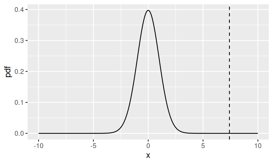
$The density of the $t_{67}$ distribution. The dashed line shows the observed value of the test statistic for the weight gain data.$

Figure 4.3: The density of the $t_{67}$ distribution. The dashed line shows the observed value of the test statistic for the weight gain data.

Example 4.13 (Fast food waiting times) Suppose the manager of the fast food outlet claims that the average waiting time is only 60 seconds. So, we want to test $H_{0}: \mu=60$. We have $n=20, \bar{x}=67.85, s=18.36$. Hence our test statistic for the null hypothesis $H_{0}: \mu=\mu_{0}=60$ is \[\sqrt{n} \frac{\left(\bar{x}-\mu_{0}\right)}{s}=\sqrt{20} \frac{(67.85-60)}{18.36}=1.91.\]

The observed value of $1.91$ may or may not be reasonable from Figure 4.4, which shows the density of the $t$-distribution with 19 degrees of freedom, and a vertical line at the observed value of $1.91$. This value is a bit out in the tail but we are not sure, unlike in the previous weight gain example. So how can we decide whether to reject the null hypothesis?

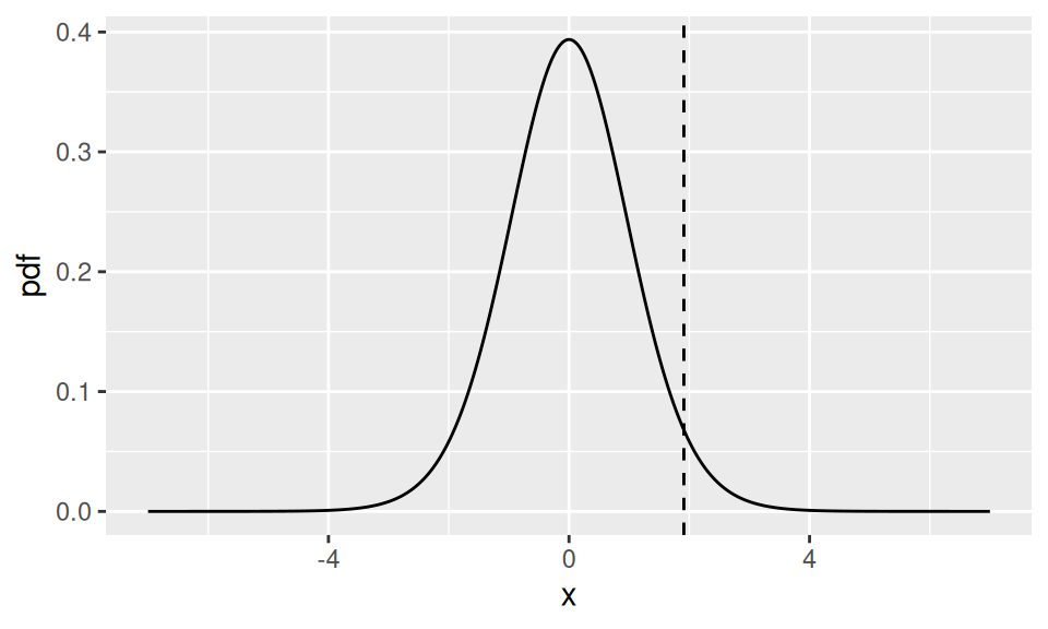
$The density of the $t_{19}$ distribution. The dashed line shows the observed value of the test statistic for the fast food data.$

Figure 4.4: The density of the $t_{19}$ distribution. The dashed line shows the observed value of the test statistic for the fast food data.

4.5.2.2 The significance level

The significance level $\alpha$ is the Type I error rate. Smaller $\alpha$ reduces false rejections but increases the chance of failing to reject poor models (Type II error). A common choice is $\alpha=0.05$; we reject when the test statistic falls in a region of total null probability $\alpha$.

4.5.2.3 Rejection region

For the t-test, the null distribution is $t_{n-1}$ where $n$ is the sample size, so the rejection region for the test corresponds to a region of total probability $\alpha=0.05$ comprising the ‘most extreme’ values in the direction of the alternative hypothesis. If the alternative hypothesis is two-sided, e.g. $H_{1}: \mu \neq \mu_{0}$, then this is obtained as below, where the two shaded regions both have area (probability) $\alpha / 2=0.025$.

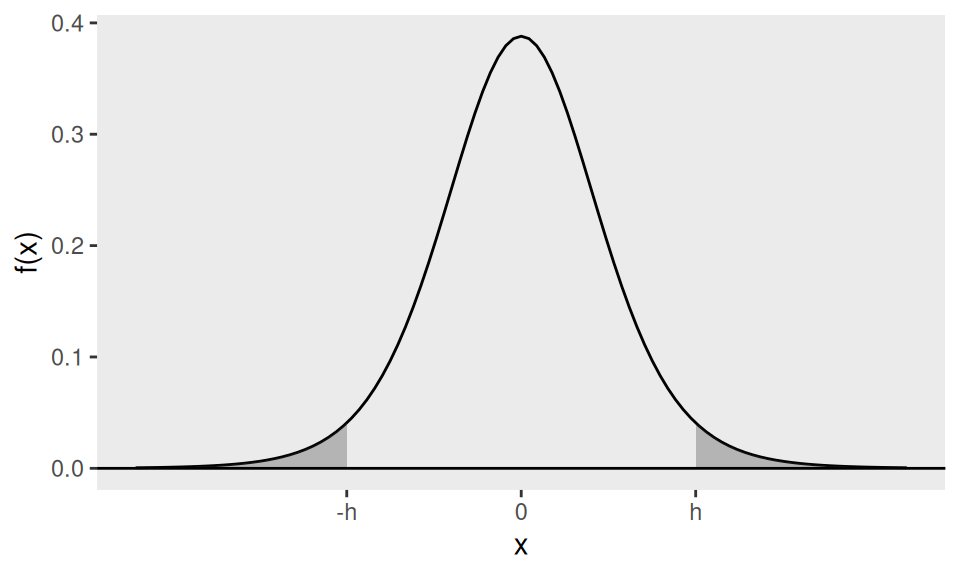
$The shaded area shows the rejection region for a t-test. $h$ is chosen to make the shaded area equal to the significance level $1-\alpha$$

Figure 4.5: The shaded area shows the rejection region for a t-test. $h$ is chosen to make the shaded area equal to the significance level $1-\alpha$

The value of $h$ depends on the sample size $n$ and can be found in R with the qt command. Note that we need to put $n-1$ in the df argument of qt. So for $n = 100$, we can find $h$ with

qt(0.975, df = 99)

## [1] 1.984217

For some other values of $n$, we have

where the last value for $n=\infty$ is obtained from the normal distribution.

For a one-sided alternative (e.g., $H_{1}:\mu>\mu_{0}$), the rejection region lies in the right tail: reject if the statistic exceeds $h$, chosen so that the right-tail area under $t_{n-1}$ is $\alpha$. So for $n = 100$ and $\alpha = 0.05$, we can find this $h$ with

qt(0.95, df = 99)

## [1] 1.660391

For some other values of $n$, we have

4.5.2.4 Summary of the t-test procedure

Compute the test statistic \[t=\sqrt{n} \frac{\left(\bar{x}-\mu_{0}\right)}{s}.\]
For a chosen $\alpha$ (usually 0.05), the two-sided rejection region is $|t|>h$, where $-h$ is the $\alpha/2$ percentile of $t_{n-1}$.
If your computed $t$ lies in the rejection region, i.e. $|t|>h$, you report that $H_{0}$ is rejected in favour of $H_{1}$ at the chosen level of significance. If $t$ does not lie in the rejection region, you report that $H_{0}$ is not rejected. (Never refer to ‘accepting’ a hypothesis.)

4.5.2.5 Examples

Example 4.14 (Fast food waiting times) We would like to test $H_{0}: \mu=60$ against the alternative $H_{1}: \mu>60$, as this alternative will refute the claim of the store manager that customers only wait for a maximum of one minute. We calculated the observed value to be $1.91$. This is a one-sided test and for a $5 \%$ level of significance, the critical value $h$ will come from $\texttt{qt(0.95, df = 19)}=1.73$. Thus the observed value is higher than the critical value so we will reject the null hypothesis, disputing the manager’s claim regarding a minute wait.

Example 4.15 (Weight gain) For the weight gain example $\bar{x}=0.8671, s=0.9653, n=68$. Then, we would be interested in testing $H_{0}: \mu=0$ against the alternative hypothesis $H_{1}: \mu \neq 0$ in the model that the data are observations of i.i.d. $N\left(\mu, \sigma^{2}\right)$ random variables.

We obtain the test statistic \[t=\sqrt{n} \frac{\left(\bar{x}-\mu_{0}\right)}{s}=\sqrt{68} \frac{(0.8671-0)}{0.9653}=7.41.\]
Under $H_{0}$ this is an observation from a $t_{67}$ distribution. For significance level $\alpha=0.05$ the rejection region is $|t|>1.996$.
Our computed test statistic lies in the rejection region, i.e. $|t|>1.996$, so $H_{0}$ is rejected in favour of $H_{1}$ at the $5 \%$ level of significance.

In R we can perform the test as follows:

wtgain$diff <- wtgain$final - wtgain$initial
t.test(wtgain$diff)

## 
##  One Sample t-test
## 
## data:  wtgain$diff
## t = 7.4074, df = 67, p-value = 2.813e-10
## alternative hypothesis: true mean is not equal to 0
## 95 percent confidence interval:
##  0.6334959 1.1008265
## sample estimates:
## mean of x 
## 0.8671612

This yields $t=7.4074$ with $\mathrm{df}=67$.

4.5.2.6 p-values

The result of a test is most commonly summarised by rejection or non-rejection of $H_{0}$ at the stated level of significance. An alternative, which you may see in practice, is the computation of a p-value. This is the probability, under $H_0$, of observing the realised test statistic or something more extreme. Small p-values indicate evidence against $H_0$. A common threshold is 0.05.

For the t-test with a two-sided alternative, the p-value is given by:\[p=P\left(|T|>\left|t_{\text{obs}}\right|\right)=2 P\left(T>\left|t_{\text{obs}}\right|\right),\] where $T$ has a $t_{n-1}$ distribution and $t_{\text{obs }}$ is the observed sample value.

However, if the alternative is one-sided and to the right then the p-value is given by: \[p=P\left(T>t_{\text{obs}}\right),\] where $T$ has a $t_{n-1}$ distribution and $t_{\text{obs}}$ is the observed sample value.

A small p-value corresponds to an observation of $T$ that is improbable (since it is far out in the low probability tail area) under $H_{0}$ and hence provides evidence against $H_{0}$. The p-value should not be misinterpreted as the probability that $H_{0}$ is true. $H_{0}$ is not a random event (under our models) and so cannot be assigned a probability. The null hypothesis is rejected at significance level $\alpha$ if the p-value for the test is less than $\alpha$. \[\text { Reject } H_{0} \text { if p-value }<\alpha.\]

Example 4.16 (Fast food waiting times) In the fast food example, a test of $H_{0}: \mu=60$ resulted in a test statistic $t=1.91$. Then the p-value is given by \[p=P(T>1.91)=0.036 \text {, when } T \sim t_{19}.\]

This is the area of the shaded region in Figure 4.6. In R it is

1 - pt(1.91, df = 19)

## [1] 0.03567359

The p-value $0.036$ indicates some evidence against the manager’s claim at the $5 \%$ level of significance but not the $1 \%$ level of significance.

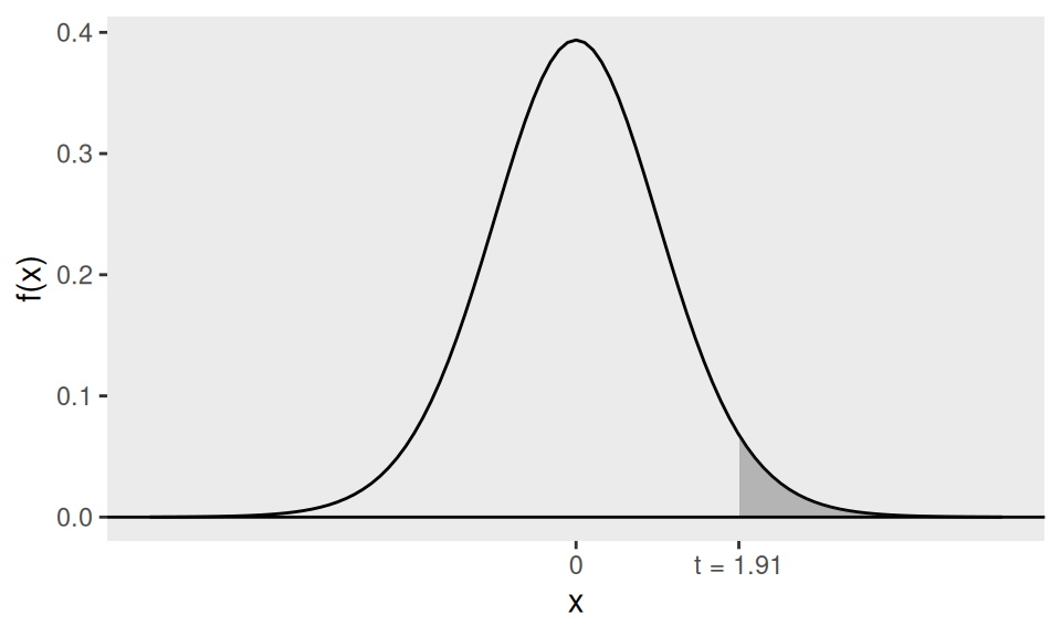
$The area of the shaded region (under the $t_{19}$ pdf) is the p-value for the one-sided hypothesis test in the fast food example$

Figure 4.6: The area of the shaded region (under the $t_{19}$ pdf) is the p-value for the one-sided hypothesis test in the fast food example

When the alternative hypothesis is two-sided the p-value has to be calculated from $P\left(|T|>t_{\text {obs }}\right)$, where $t_{\text {obs }}$ is the observed value and $T$ follows the $t$-distribution with $n-1$ df.

Example 4.17 (Weight gain) Because the alternative is two-sided, the p-value is given by: \[p=P(|T|>7.41)=2.78 \times 10^{-10} \approx 0.0, \text { when } T \sim t_{67}.\] This very small p-value indicates very strong evidence against the null hypothesis of no weight gain in the first year of college.

4.5.2.7 Equivalence of testing and interval estimation

Note that the $95 \%$ confidence interval for $\mu$ in the weight gain example has previously been calculated to be $(0.6335,1.1008)$ in Example 4.9. This interval does not include the hypothesised value 0 of $\mu$. Hence we can conclude that the hypothesis test at the $5 \%$ level of significance will reject the null hypothesis $H_{0}: \mu=0$.

This is because \[\left|T_\text{obs}=\frac{\sqrt{n}\left(\bar{x}-\mu_{0}\right)}{s}\right|>h\] implies and is implied by $\mu_{0}$ being outside the interval \[(\bar{x}-h s / \sqrt{n}, \bar{x}+h s / \sqrt{n}).\] Notice that $h$ is the same in both. For this reason we often just calculate the confidence interval and take the reject/do not reject decision merely by inspection.

4.5.3 Two sample t-tests

Suppose we observe two samples $x_{1}, \ldots, x_{n}$ and $y_{1}, \ldots, y_{m}$, modelled as \[X_{1}, \ldots, X_{n} \stackrel{\text{ i.i.d. }}{\sim} N\left(\mu_{X}, \sigma_{X}^{2}\right)\] and \[Y_{1}, \ldots, Y_{m} \stackrel{\text { i.i.d. }}{\sim} N\left(\mu_{Y}, \sigma_{Y}^{2}\right)\] respectively, where it is also assumed that the $X$ and $Y$ variables are independent of each other. Suppose that we want to test the hypothesis that the distributions of $X$ and $Y$ are identical, that is \[H_{0}: \mu_{X}=\mu_{Y}, \quad \sigma_{X}=\sigma_{Y}=\sigma\] against the alternative hypothesis \[H_{1}: \mu_{X} \neq \mu_{Y}.\]

In Chapter 3 we proved that \[\bar{X} \sim N\left(\mu_{X}, \sigma_{X}^{2} / n\right) \text { and } \bar{Y} \sim N\left(\mu_{Y}, \sigma_{Y}^{2} / m\right)\] and therefore \[\bar{X}-\bar{Y} \sim N\left(\mu_{X}-\mu_{Y}, \frac{\sigma_{X}^{2}}{n}+\frac{\sigma_{Y}^{2}}{m}\right).\]

Hence, under $H_{0}$, \[\bar{X}-\bar{Y} \sim N\left(0, \sigma^{2}\left[\frac{1}{n}+\frac{1}{m}\right]\right) \Rightarrow \sqrt{\frac{n m}{n+m}} \frac{(\bar{X}-\bar{Y})}{\sigma} \sim N(0,1).\]

The involvement of the (unknown) $\sigma$ above means that this is not a pivotal test statistic. It will be proved in Statistical Inference that if $\sigma^2$ is replaced by its unbiased estimator $S^2$, which here is the two-sample estimator of the common variance, given by \[S^{2}=\frac{\sum_{i=1}^{n}\left(X_{i}-\bar{X}\right)^{2}+\sum_{i=1}^{m}\left(Y_{i}-\bar{Y}\right)^{2}}{n+m-2},\] then \[\sqrt{\frac{n m}{n+m}} \frac{(\bar{X}-\bar{Y})}{S} \sim t_{n+m-2}.\] Hence \[t=\sqrt{\frac{n m}{n+m}} \frac{(\bar{x}-\bar{y})}{s}\] is a test statistic. For a two-sided test, reject if $|t|>h$, where $-h$ is the $\alpha/2$ percentile of $t_{n+m-2}$.

From the hypothesis testing, a $100(1-\alpha) \%$ confidence interval for $\mu_{X}-\mu_{Y}$ is given by \[\bar{x}-\bar{y} \pm h \sqrt{\frac{n+m}{n m}} s,\] where $-h$ is the $\alpha / 2$ (usually $0.025$ ) percentile of $t_{n+m-2}$.

Example 4.18 (Fast food waiting times) In this example, we would like to know if there are significant differences between the AM and PM waiting times. Here $n=m=10$, $\bar{x}=68.9$, $\bar{y}=66.8$, $s_{x}^{2}=538.22$ and $s_{y}^{2}=171.29$. From this we calculate, \[s^{2}=\frac{(n-1) s_{x}^{2}+(m-1) s_{y}^{2}}{n+m-2}=354.8,\] and \[t_{\text{obs}}=\sqrt{\frac{n m}{n+m}} \frac{(\bar{x}-\bar{y})}{s}=0.25.\] This is not significant as the critical value $h = \texttt{qt(0.975, df = 18)}=2.10$ is larger in absolute value than $0.25$. We can conduct the test easily in R:

fastfood_am <- c(38, 100, 64, 43, 63, 59, 107, 52, 86, 77)
fastfood_pm <- c(45, 62, 52, 72, 81, 88, 64, 75, 59, 70)
t.test(fastfood_am, fastfood_pm)

## 
##  Welch Two Sample t-test
## 
## data:  fastfood_am and fastfood_pm
## t = 0.24929, df = 14.201, p-value = 0.8067
## alternative hypothesis: true difference in means is not equal to 0
## 95 percent confidence interval:
##  -15.9434  20.1434
## sample estimates:
## mean of x mean of y 
##      68.9      66.8

R reports the test statistic ($0.249$), p-value ($0.8067$), and the 95% CI $(-15.94, 20.14)$.

4.5.4 Paired t-test

Sometimes $X$ and $Y$ are not independent by design, e.g., paired measurements on the same subjects before $(X)$ and after $(Y)$ treatment (as in the weight gain example). In such cases, analyse the differences \[z_{i}=x_{i}-y_{i}, \quad i=1, \ldots, n\] and modelling these differences as observations of i.i.d. $N\left(\mu_{z}, \sigma_{Z}^{2}\right)$ variables $Z_{1}, \ldots, Z_{n}$. Then, a test of the hypothesis $\mu_{X}=\mu_{Y}$ is achieved by testing $\mu_{Z}=0$, which is just a standard (one sample) t-test, as described previously.

Example 4.19 Water-quality researchers wish to measure the biomass to chlorophyll ratio for phytoplankton (in milligrams per litre of water). There are two possible tests, one less expensive than the other. To see whether the two tests give the same results, ten water samples were taken and each was measured both ways. The results are as follows:

To test the null-hypothesis \[H_{0}: \mu_{Z}=0 \text { against } H_{1}: \mu_{Z} \neq 0\] we use the test statistic $t=\sqrt{n} \frac{\bar{z}}{s_{z}}$, where $s_{z}^{2}=\frac{1}{n-1} \sum_{i=1}^{n}\left(z_{i}-\bar{z}\right)^{2}$.

From the hypothesis testing, a $100(1-\alpha) \%$ confidence interval for $\mu_Z$ is given by $\bar{z} \pm h \frac{s_{z}}{\sqrt{n}}$, where $h$ is the critical value of the $t$ distribution with $n-1$ degrees of freedom. In R we perform the test as follows:

x <- c(45.9, 57.6, 54.9, 38.7, 35.7, 39.2, 45.9, 43.2, 45.4, 54.8)
y <- c(48.2, 64.2, 56.8, 47.2, 43.7, 45.7, 53.0, 52.0, 45.1, 57.5)

t.test(x, y, paired = TRUE)

## 
##  Paired t-test
## 
## data:  x and y
## t = -5.0778, df = 9, p-value = 0.0006649
## alternative hypothesis: true mean difference is not equal to 0
## 95 percent confidence interval:
##  -7.531073 -2.888927
## sample estimates:
## mean difference 
##           -5.21

This gives the test statistic $t_{\text{obs}}=-5.0778$ with a df of 9 and a p-value $=0.0006649$. Thus we reject the null hypothesis. The associated $95 \%$ CI is $(-7.53,-2.89)$.

The second test yields significantly higher values than the first, so it cannot replace the first.

MATH1063: Introduction to Statistics