3.1 Basic nonlinear models
So far we have only considered models where the link function of the mean response is equal to the linear predictor, i.e. in the most general case of the generalised linear mixed model (GLMM) \[\mu_{ij} = E(y_{ij}), \qquad g(\mu_{ij}) = \eta_{ij} = x_{ij}^T \beta + z_{ij}^T b_i,\] and where the response distribution for \(y\) is from the exponential family of distributions. The key point is that the linear predictor is a linear function of the parameters. Linear models, generalised linear models (GLMs) and linear mixed models (LMMs) are all special cases of the GLMM.
These “linear” models form the basis of most applied statistical analyses. Usually, there is no scientific reason to believe these linear models are true for a given application.
We begin by considering nonlinear extensions of the normal linear model \[\begin{equation} y_i = x_i^T \beta + \epsilon_i, \tag{3.1} \end{equation}\] where \(\epsilon_i \sim N(0,\sigma^2)\), independently, where \(\beta\) are the \(p\) regression parameters. Instead of the mean response being the linear predictor \(x_i^T \beta\), we could allow it to be a nonlinear function of parameters, i.e. \[\begin{equation} y_i = \eta(x_i, \beta) + \epsilon_i, \tag{3.2} \end{equation}\] where \(\epsilon_i \sim N(0,\sigma^2)\), independently, where \(\beta\) are the \(p\) nonlinear parameters. The model specified by (3.2) has the linear model (3.1) as a special case when \(\eta(x, \beta) = x^T \beta\).
Nonlinear parameters can be of two different types:
- Physical parameters have meaning within the science underlying the model, \(\eta(x, \beta)\). Estimating the value of physical parameters contributes to scientific understanding.
- Tuning parameters do not have physical meaning. Their presence is often as a simplification of a more complex underlying system. Their estimation is to make the model fit best to reality.
How might the function \(\eta(x, \beta)\) be specified?
- Mechanistically – prior scientific knowledge is incorporated into building a mathematical model for the mean response. This can often be complex and \(\eta(x, \beta)\) may not be available in closed form.
- Phenomenologically (empirically) – a function \(\eta(x, \beta)\) may be posited that appears to capture the non-linear nature of the mean response.
Example 3.1
The response, \(y\), is the uptake of calcium (in nmoles per mg) at time \(x\) (in minutes) by \(n=27\) cells in “hot” suspension. Figure 3.1 shows calcium uptake against time.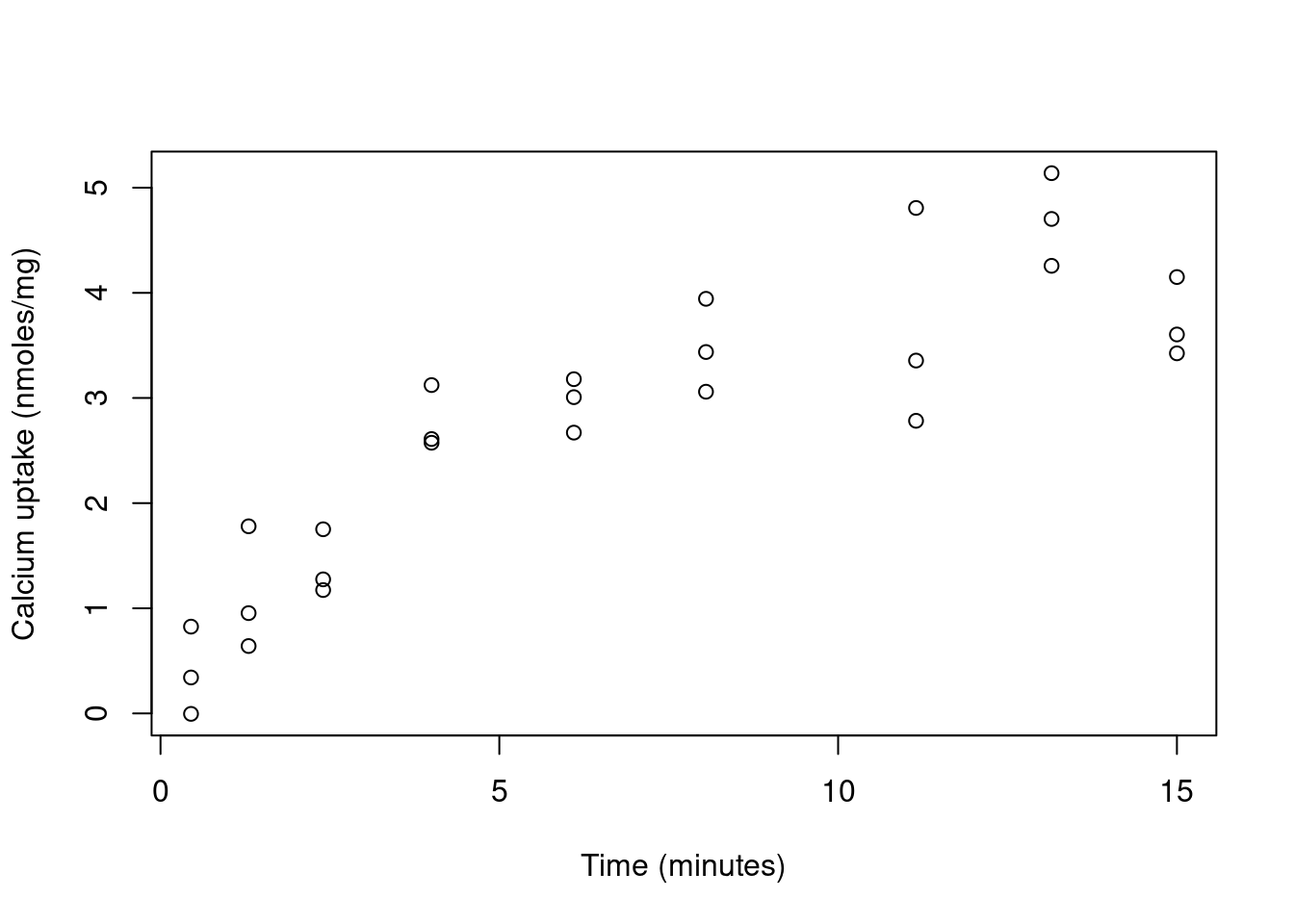
Figure 3.1: Calcium uptake against time
We see that calcium uptake “grows” with time. There is a large class of phenomenological models for growth curves. Consider the non-linear model with \[\begin{equation} \eta(x, \beta) = \beta_0 \left( 1 - \exp \left( - x / \beta_1 \right) \right). \tag{3.3} \end{equation}\] This is derived by assuming that the rate of growth is proportional to the calcium remaining, i.e. \[\frac{d \eta}{d x} = (\beta_0 - \eta)/\beta_1.\] The solution (with initial condition \(\eta(0,\beta)=0\)) to this differential equation is (3.3). Here \(\beta_0\) is the final size of the population, and \(\beta_1\) (inversely) controls the growth rate.
Figure 3.2 shows fitted lines for the three different models added to the plot of calcium uptake against time.
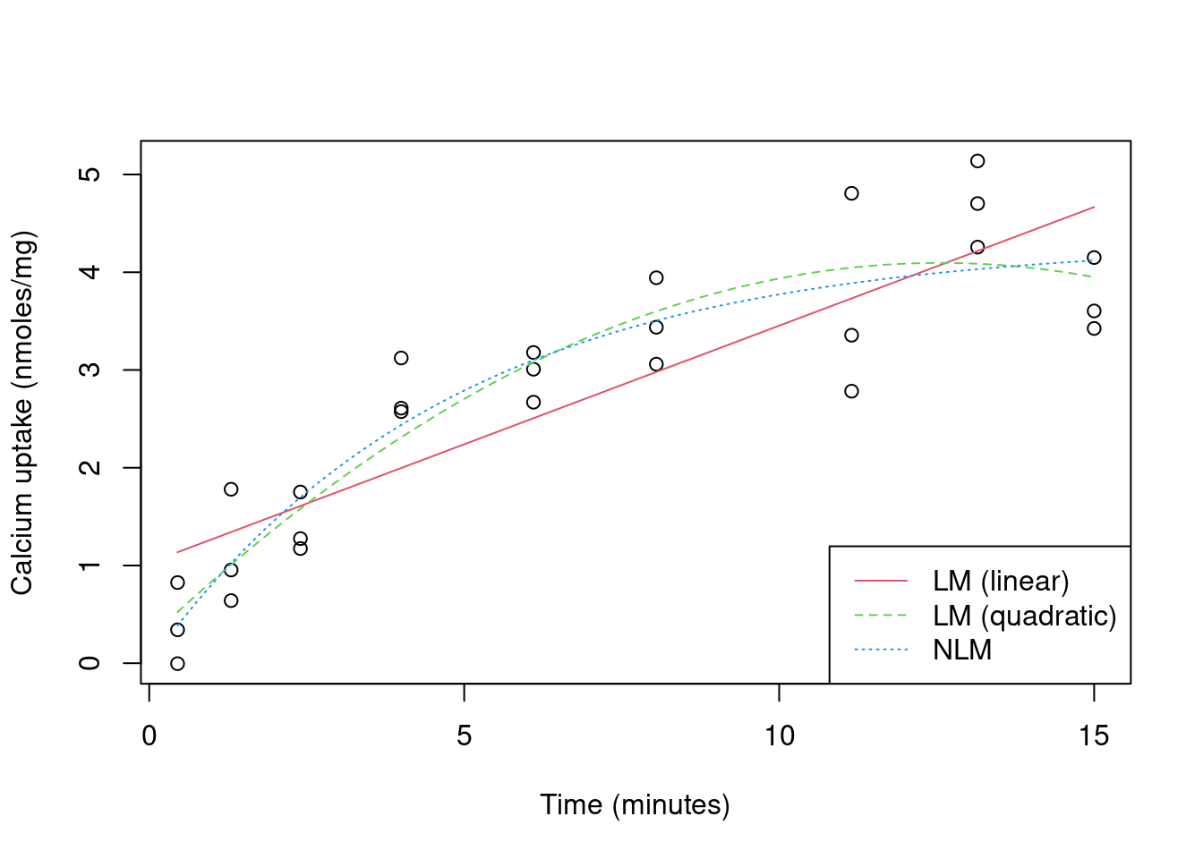
Figure 3.2: Calcium uptake against time, with expected uptake from three models overlaid
A comparison of the goodness-of-fit for the three models is shown in Table 3.1. The goodness-of-fit for the quadratic and nonlinear models is identical (to 2 decimal places). Since the nonlinear model is simpler (fewer parameters), it is the preferred model.
| Model | Parameters (\(p\)) | \(l(\hat{\beta})\) | AIC |
|---|---|---|---|
| Linear model (slope) | 2 | -28.70 | 63.40 |
| Linear model (quadratic) | 3 | -20.95 | 49.91 |
| Non-linear model | 2 | -20.95 | 47.91 |