1.1 Introduction

$ \newcommand{\bm}[1]{\boldsymbol{\mathbf{#1}}} \DeclareMathOperator{\tr}{tr} \DeclareMathOperator{\var}{var} \DeclareMathOperator{\cov}{cov} \DeclareMathOperator{\corr}{corr} \newcommand{\indep}{\perp\!\!\!\perp} \newcommand{\nindep}{\perp\!\!\!\perp\!\!\!\!\!\!/\;\;} $

All models are wrong, but some models are useful

– George Box (1919–2013)

Statisticians construct models to simplify reality, to gain understanding, to compare scientific, economic, or other theories, and to predict future events or data. We rarely believe in our models, but regard them as temporary constructs, which should be subject to improvement. Often we have several models and must decide which, if any, is preferable.

Criteria for model selection include:

Substantive knowledge, from previous studies, theoretical arguments, dimensional or other general considerations.
Sensitivity to failure of assumptions: we prefer models that provide valid inference even if some of their assumptions are invalid.
Quality of fit of models to data: we could use informal measures such as residuals, graphical assessment, or more formal or goodness-of-fit tests.
For reasons of economy we seek ‘simple’ models.

There may be a very large number of plausible models for us to compare. For instance, in a linear regression with $p$ covariates, there are $2^p$ possible combinations of covariates: for each covariate, we need to decide whether or not to include that variable in the model. If $p=20$ we have over a million possible models to consider, and the problem becomes even more complex if we allow for transformations and interactions in the model.

To focus and simplify discussion we will consider model selection among parametric models, but the ideas generalise to semi-parametric and non-parametric settings.

Example 1.1 A logistic regression model for binary responses assumes that $Y_i \sim \text{Bernoulli}(\pi_i)$, with a linear model for log odds of ‘success’ \[\log\left\{\frac{P(Y_i=1)}{P(Y_i=0)}\right\}= \log\left(\frac{\pi_i}{1-\pi_i}\right) = x_i^T\beta.\] The log-likelihood for $\beta$ based on independent responses with covariate vectors $x_1, \ldots, x_n$ is \[\ell(\beta) = \sum_{j=1}^n y_jx_j^T \beta - \sum_{j=1}^n \log\left\{1 + \exp( x_j^T \beta)\right\}\] A good fit gives large fitted loglikelihood $\hat \ell = \ell(\hat\beta)$ where $\hat\beta$ is the MLE under the model.

The SMPracticals package contains a dataset called nodal, which relates to the the nodal involvement (r) of 53 patients with prostate cancer, with five binary covariates aged, stage, grade, xray and acid. Considering only of models without any interaction between the 5 binary covariates, there are still $2^5 = 32$ possible logistic regression models for this data. We can rank these models according to fitted loglikelihood $\hat \ell$. Figure 1.1 summarises this as a plot of the number of parameters against the fitted loglikelihood for each of the 32 models under consideration.

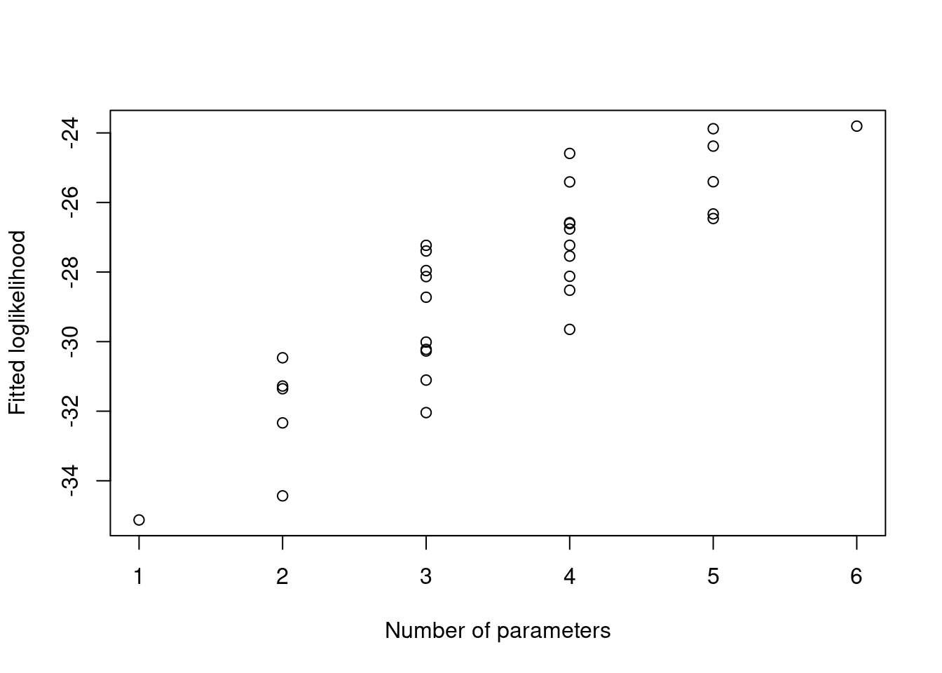
$Fitted loglikelihood for 32 possible logistic regression models for the \texttt{nodal} data$

Figure 1.1: Fitted loglikelihood for 32 possible logistic regression models for the data

Adding terms always increases the loglikelihood $\hat\ell$, so taking the model with highest $\hat\ell$ would give the full model. We need to a different way to compare models, which should trade off quality of fit (measured by $\hat \ell$) and model complexity (number of parameters).