2.3 Dependence
2.3.1 Toxoplasmosis example revisited
Example 2.3 We can think of the toxoplasmosis proportions \(Y_i\) in each city (\(i\)) as arising from the sum of binary variables, \(Y_{ij}\), representing the toxoplasmosis status of individuals (\(j\)), so \(m_iY_i=\sum_{j=1}^{m_i} Y_{ij}\).
Then \[\begin{align*} \var(Y_i)&=\frac{1}{m_i^2}\sum_{j=1}^{m_i} \var(Y_{ij}) +\frac{1}{m_i^2}\sum_{j\not = k} \cov(Y_{ij},Y_{ik})\\ &=\frac{\mu_i(1-\mu_i)}{m_i} +\frac{1}{m_i^2}\sum_{j\not = k} \cov(Y_{ij},Y_{ik}) \end{align*}\]
So any positive correlation between individuals induces overdispersion in the counts.
There may be a number of plausible reasons why the responses corresponding to units within a given cluster are dependent (in the toxoplasmosis example, cluster \(=\) city). One compelling reason is the unobserved heterogeneity discussed previously.
In the ‘correct’ model (corresponding to \(\eta_i^\text{true}\)), the toxoplasmosis status of individuals, \(Y_{ij}\), are independent, so \[Y_{ij}\indep Y_{ik}\mid \eta_i^\text{true}\quad\Leftrightarrow\quad Y_{ij}\indep Y_{ik}\mid \eta_i^\text{model}, \eta_i^\text{diff}.\] However, in the absence of knowledge of \(\eta_i^\text{diff}\) \[\quad Y_{ij}\nindep Y_{ik}\mid \eta_i^\text{model}.\] Hence conditional (given \(\eta_i^\text{diff}\)) independence between units in a common cluster \(i\) becomes marginal dependence, when marginalised over the population distribution \(F\) of unobserved \(\eta_i^\text{diff}\).
The correspondence between positive intra-cluster correlation and unobserved heterogeneity suggests that intra-cluster dependence might be modelled using random effects, For example, for the individual-level toxoplasmosis data \[Y_{ij}\sim \text{Bernoulli}(\mu_{ij}),\quad \log \frac{\mu_{ij}}{1-\mu_{ij}}=x_{ij}^T\beta+u_i,\quad u_i\sim N(0,\sigma^2)\] which implies \[\quad Y_{ij}\nindep Y_{ik}\mid \beta,\sigma^2\]
Intra-cluster dependence arises in many applications, and random effects provide an effective way of modelling it.2.3.2 Marginal models and generalised estimating equations
Random effects modelling is not the only way of accounting for intra-cluster dependence.
A marginal model models \(\mu_{ij}\equiv E(Y_{ij})\) as a function of explanatory variables, through \(g(\mu_{ij})=x_{ij}^T\beta\), and also specifies a variance relationship \(\var(Y_{ij})=\sigma^2V(\mu_{ij})/m_{ij}\) and a model for \(\corr(Y_{ij},Y_{ik})\), as a function of \(\mu\) and possibly additional parameters.
It is important to note that the parameters \(\beta\) in a marginal model have a different interpretation from those in a random effects model, because for the latter \[E(Y_{ij})=E(g^{-1}[x_{ij}^T\beta+u_i])\not = g^{-1}(x_{ij}^T\beta)\quad \text{(unless $g$ is linear)}.\]
A random effects model describes the mean response at the subject level (‘subject specific’). A marginal model describes the mean response across the population (‘population averaged’).
As with the quasi-likelihood approach above, marginal models do not generally provide a full probability model for \(Y\). Nevertheless, \(\beta\) can be estimated using generalised estimating equations (GEEs).
The GEE for estimating \(\beta\) in a marginal model is of the form \[\sum_i \left(\frac{\partial\mu_i}{\partial\beta}\right)^T\var(Y_i)^{-1}(Y_i-\mu_i)=0\] where \(Y_i=(Y_{ij})\) and \(\mu_i=(\mu_{ij})\).
Consistent covariance estimates are available for GEE estimators. Furthermore, the approach is generally robust to mis-specification of the correlation structure. For the rest of this module, we focus on fully specified probability models.
2.3.3 Clustered data
Examples where data are collected in clusters include:
- Studies in biometry where repeated measures are made on experimental units. Such studies can effectively mitigate the effect of between-unit variability on important inferences.
- Agricultural field trials, or similar studies, for example in engineering, where experimental units are arranged within blocks.
- Sample surveys where collecting data within clusters or small areas can save costs.
Of course, other forms of dependence exist, for example spatial or serial dependence induced by arrangement in space or time of units of observation.
Example 2.4
Therat.growth data in SMPracticals
gives the weekly weights (y) of 30 young rats.
Figure 2.2 shows the weight against week separately for each rat.
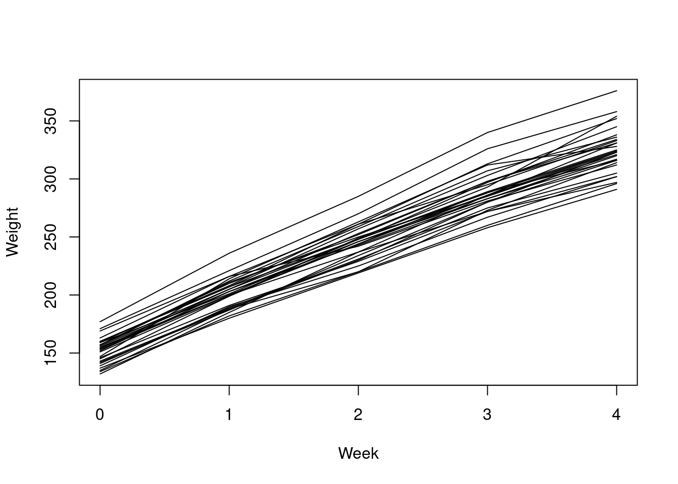
Figure 2.2: Individual rat weight by week, for the rat growth data
Writing \(y_{ij}\) for the \(j\)th observation of the weight of rat \(i\), and \(x_{ij}\) for the week in which this record was made, we can fit the simple linear regression \[y_{ij}=\beta_0+\beta_1 x_{ij}+\epsilon_{ij}\] with resulting estimates \(\hat\beta_0=156.1\) (2.25) and \(\hat\beta_1=43.3\) (0.92). Figure 2.3 shows the residuals from this model, separately for each rat, showing clear evidence of an unexplained difference between rats.
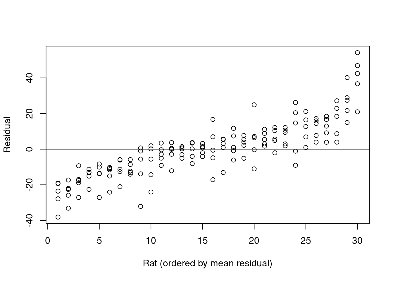
Figure 2.3: Residuals from a simple linear regression for each rat in the rat.growth data