3.2 Extending the nonlinear model
3.2.1 Introduction
Nonlinear models can be extended to non-normal responses and clustered responses in the same way as linear models. Here, we consider clustered responses and briefly discuss the nonlinear mixed model.
Example 3.2
Theophylline is an anti-asthmatic drug. An experiment was performed on \(n=12\) individuals to investigate the way in which the drug leaves the body. The study of drug concentrations inside organisms is called pharmacokinetics. An oral dose, \(D_i\), was given to the \(i\)th individual at time \(t=0\), for \(i=1,\dots,n\). The concentration of theophylline in the blood was then measured at 11 time points in the next 25 hours. Let \(y_{ij}\) be the theophylline concentration (mg/L) for individual \(i\) at time \(t_{ij}\). Figure 3.3 shows the concentration of theophylline against time for each of the individuals. There is a sharp increase in concentration followed by a steady decrease.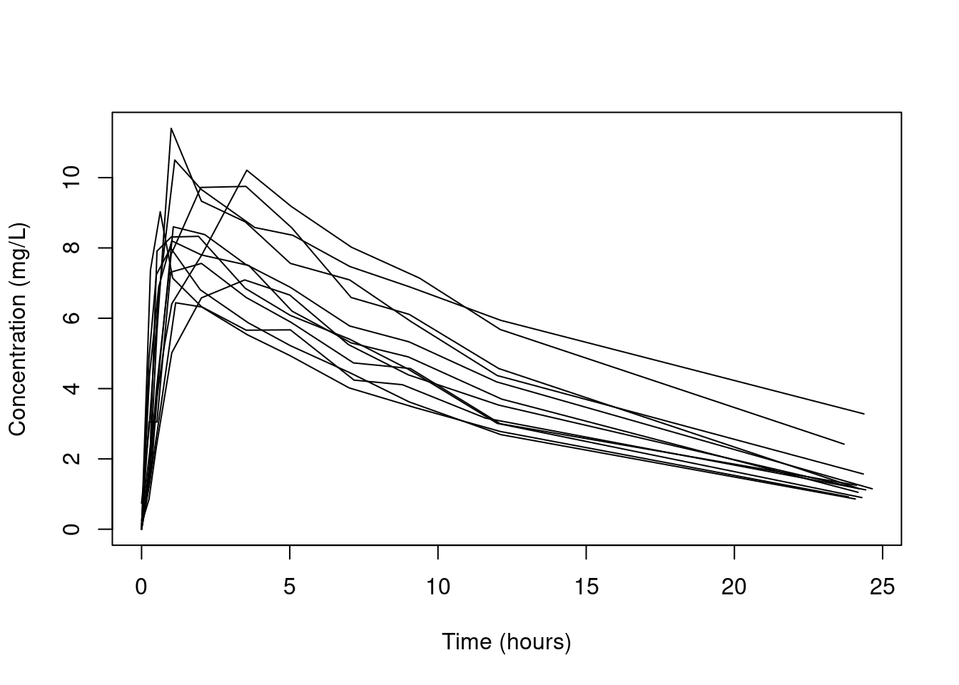
Figure 3.3: Concentration of theophylline against time for each of the individuals in the study
Compartmental models are a common class of model used in pharmacokinetics studies. If the initial dosage is \(D\), then a two-compartment open pharmacokinetic model is \[\eta(\beta, D,t) = \frac{D \beta_1 \beta_2}{\beta_3(\beta_2 - \beta_1)} \left( \exp \left( - \beta_1 t\right) - \exp \left( - \beta_2 t\right)\right),\] where the (positive) nonlinear parameters are
- \(\beta_1\), the elimination rate which controls the rate at which the drug leaves the organism;
- \(\beta_2\), the absorption rate which controls the rate at which the drug enters the blood;
- \(\beta_3\), the clearance which controls the volume of blood for which a drug is completely removed per time unit.
Initially ignore the dependence induced from repeated measurements on individuals and assume the following basic nonlinear model \[y_{ij} = \eta(\beta, D_i,t_{ij}) + \epsilon_{ij},\] where \(\epsilon_{ij} \sim N(0,\sigma^2)\). Figure 3.4 gives a plot of the residuals for each subject in the study under this model, showing evidence of an unexplained difference between individuals.
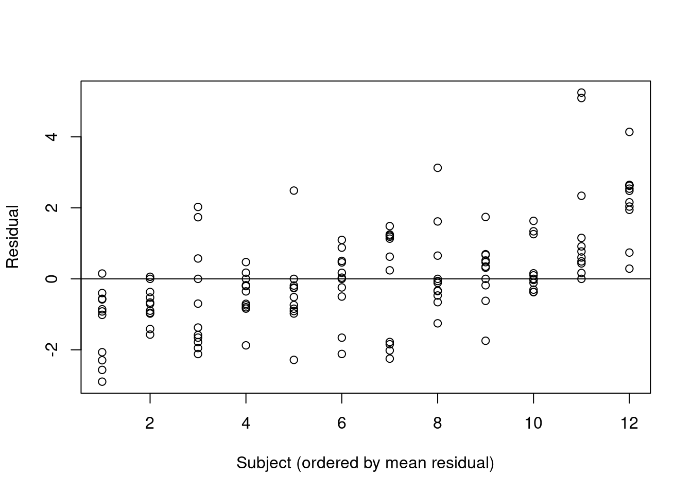
Figure 3.4: Residuals for each individual in the theopylline study, assuming a basic nonlinear model which ignores dependence
3.2.2 Nonlinear mixed effects models
A nonlinear mixed model is \[y_{ij} = \eta(\beta + b_i, x_{ij}) + \epsilon_{ij},\] where \[\epsilon_{ij} \sim N(0,\sigma^2), \qquad b_i \sim N(0,\Sigma_b),\] and \(\Sigma_b\) is a \(q \times q\) covariance matrix.
This model specifies that \(\beta_i = \beta + b_i\) are the nonlinear parameters for the \(i\)th cluster, i.e. the cluster-specific nonlinear parameters. In the case of the Theophylline example, each individual would have unique elimination rate, absorption rate and clearance. It follows that \(\beta_i \sim N(\beta, \Sigma_b)\). The mean, \(\beta\), of the cluster-specific nonlinear parameters across all individuals are the population nonlinear parameters.
We might like to specify the model in a way such that only a subset of the nonlinear parameters can be different for each individual, and the remainder fixed for all individuals.
Suppose \(q \le p\) nonlinear parameters are can be different for each individual, then a more general way of writing the nonlinear mixed model is \[y_{ij} = \eta(\beta + A b_i, x) + \epsilon_{ij},\] where \(\epsilon_{ij} \sim N(0,\sigma^2)\) and \(b_i \sim N(0,\Sigma_b).\) Here \(\Sigma_b\) is a \(q \times q\) covariance matrix and \(A\) is a \(p \times q\) binary matrix. \(A\) allows the specification of the fixed and varying nonlinear parameters.
The linear mixed model is a special case of the nonlinear mixed model where \[ \eta(\beta, x) = x^T \beta.\] Then \[\eta(\beta + A b, x)= x^T \left( \beta + Ab\right) = x^T \beta + x^T A b,\] so \(z = A^T x\). For a random intercept model, where \(q=1\), \(A = \left(1, 0, \dots, 0 \right)\).
Example 3.3 We fit the nonlinear mixed model, allowing all of the nonlinear parameters to vary across individuals, i.e. \(A = I_3\).
Estimates: \[\begin{array}{lcllcl} \hat{\beta}_1 &=& 0.0864 & \hat{\Sigma}_{b11} & = & 0.0166\\ \hat{\beta}_2 &=& 1.6067 & \hat{\Sigma}_{b22} & = & 0.9349\\ \hat{\beta}_3 &=& 0.0399 & \hat{\Sigma}_{b33} & = & 0.0491 \end{array}\]
We have \(\text{AIC} = 372.6\).The estimated value of \(\Sigma_{b11}\) is “small” so we fit the nonlinear mixed model, allowing absorption rate and clearance to vary across individuals, i.e. \[A = \left(\begin{array}{cc} 0 & 0 \\ 1 & 0 \\ 0 & 1 \end{array}\right).\]
Estimates: \[\begin{array}{lcllcl} \hat{\beta}_1 &=& 0.0859 & & &\\ \hat{\beta}_2 &=& 1.6032 & \hat{\Sigma}_{b22} & = & 0.6147\\ \hat{\beta}_3 &=& 0.0397 & \hat{\Sigma}_{b33} & = & 0.0284 \end{array}\]
We have \(\text{AIC} = 368.6\). No further model simplifications reduce the AIC.
3.2.3 Extensions to non-normal responses
Nonlinear models can be extended to non-normal responses in the same way as linear models. The most general model is the generalised nonlinear mixed model (GNLMM), which assumes \(y_{ij}\) is from exponential family, \[E(y_{ij}) = \mu_{ij}, \qquad g(\mu_{ij}) = \eta(\beta + A b_i, x_{ij}).\]
This model has the following special cases: \[\begin{array}{ll} \mbox{linear model} & \mbox{nonlinear model}\\ \mbox{linear mixed model} & \mbox{nonlinear mixed model}\\ \mbox{generalised linear model} & \mbox{generalised nonlinear model}\\ \mbox{generalised linear mixed model} & \end{array}\]
There are various technical and practical issues related to fitting nonlinear models (some are common to GLMs and GLMMs). For instance:
- we need to use some approximation of likelihood function (since random effects are integrated out),
- sometimes optimisation routines to find estimates do not converge to a global maximum of the likelihood,
- evaluating \(\eta(\beta, x)\) is sometimes computationally expensive.
These are all areas of current research.