2.2 Overdispersion
2.2.1 An example of overdispersion
Example 2.1 The dataset toxo in SMPracticals provides
data on the number of people testing positive
for toxoplasmosis (r) out of the number of people
tested (m) in 34 cities in El Salvador,
along with the annual rainfall in mm (rain) in those
cities.
We can fit various logistic regression models for relating toxoplasmosis incidence to rainfall. If we consider logistic models with a polynomial dependence on rainfall, AIC and stepwise selection methods both prefer a cubic model. For simplicity here, we compare the cubic model and a constant model, in which there is no dependence on rainfall.
mod_const <- glm(r/m ~ 1, data = toxo, weights = m,
                 family = "binomial")
mod_cubic <- glm(r/m ~ poly(rain, 3), data = toxo, weights = m,
                 family = "binomial")
Figure 2.1 shows the fitted proportions testing positive under the two models.
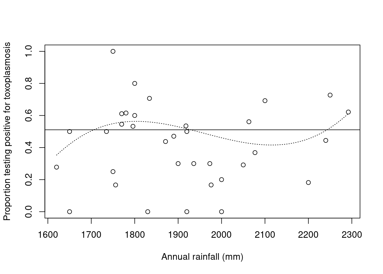
Figure 2.1: Propotion of people testing positive for toxoplasmosis against rainfall, with fitted proportions under constant (solid line) and cubic (dotted line) logistic regression models
We can conduct a hypothesis test to compare the models:
anova(mod_const, mod_cubic, test = "Chisq")## Analysis of Deviance Table
##
## Model 1: r/m ~ 1
## Model 2: r/m ~ poly(rain, 3)
## Resid. Df Resid. Dev Df Deviance Pr(>Chi)
## 1 33 74.212
## 2 30 62.635 3 11.577 0.008981 **
## ---
## Signif. codes: 0 '***' 0.001 '**' 0.01 '*' 0.05 '.' 0.1 ' ' 1There is apparently evidence to reject the null model (that there is no effect of rain on the probability of testing positive for toxoplasmosis) in favour of the cubic model.
However, we find that the residual deviance for the cubic model (\(62.63\)) is much larger than the residual degrees of freedom (\(30\)). This is an indicator of overdispersion, where the residual variability is greater than would be predicted by the specified mean/variance relationship \[\var(Y)=\frac{\mu(1-\mu)}{m}.\]
2.2.2 Quasi-likelihood
A quasi-likelihood approach to accounting for overdispersion models the mean and variance, but stops short of a full probability model for \(Y\).
For a model specified by the mean relationship \(g(\mu_i)=\eta_i=x_i^T \beta\), and variance \(\var(Y_i)= \sigma^2 V(\mu_i)/m_i\), the quasi-likelihood equations are \[\sum_{i=1}^n x_i {\frac{y_i-\mu_i}{\sigma^2 V(\mu_i) g'(\mu_i)/m_i}}=0\] If \(V(\mu_i)/m_i\) represents \(\var(Y_i)\) for a standard distribution from the exponential family, then these equations can be solved for \(\beta\) using standard GLM software.
Provided the mean and variance functions are correctly specified, asymptotic normality for \(\hat\beta\) still holds.
The dispersion parameter \(\sigma^2\) can be estimated using \[\hat\sigma^2\equiv \frac{1}{n-p-1} \sum_{i=1}^n \frac{m_i(y_i-\hat{\mu}_i)^2}{V(\hat{\mu}_i)}.\]
Example 2.2
Fitting the same models as before, but with \(\var(Y_i)=\sigma^2{\mu_i(1-\mu_i)/ m_i}\), we getmod_const_quasi <- glm(r/m ~ 1, data = toxo, weights = m,
family = "quasibinomial")
mod_cubic_quasi <- glm(r/m ~ poly(rain, 3), data = toxo, weights = m,
family = "quasibinomial")We find the estimates of the \(\beta\) coefficients are the same as before, but now we estimate \(\sigma^2\) as \(1.94\) under the cubic model.
Comparing the cubic with the constant model, we now obtain \[F=\frac{(74.21-62.62)/3}{1.94}=1.99,\]
anova(mod_const_quasi, mod_cubic_quasi, test = "F")## Analysis of Deviance Table
##
## Model 1: r/m ~ 1
## Model 2: r/m ~ poly(rain, 3)
## Resid. Df Resid. Dev Df Deviance F Pr(>F)
## 1 33 74.212
## 2 30 62.635 3 11.577 1.9888 0.1369After accounting for overdispersion, there is much less compelling evidence in favour of an effect of rainfall on toxoplasmosis incidence.
2.2.3 Models for overdispersion
To construct a full probability model in the presence of overdispersion, it is necessary to consider why overdispersion might be present.
Possible reasons include:
- There may be an important explanatory variable, other than rainfall, which we haven’t observed.
- Or there may be many other features of the cities, possibly unobservable, all having a small individual effect on incidence, but a larger effect in combination. Such effects may be individually undetectable – sometimes described as natural excess variability between units.
When part of the linear predictor is ‘missing’ from the model, \[\eta_i^\text{true}=\eta_i^\text{model}+\eta_i^\text{diff}.\] We can compensate for this, in modelling, by assuming that the missing \(\eta_i^\text{diff} \sim F\) in the population. Hence, given \(\eta_i^\text{model}\) \[ \mu_i\equiv g^{-1}(\eta_i^\text{model}+\eta_i^\text{diff})\sim G\] where \(G\) is the distribution induced by \(F\). Then \[E(Y_i)=E_G[E(Y_i\mid \mu_i)]=E_G(\mu_i)\] \[\var(Y_i)=E_G(V(\mu_i)/m_i)+\var_G(\mu_i)\]
One approach is to model the \(Y_i\) directly, by specifying an appropriate form for \(G\).
For example, for the toxoplasmosis data, we might specify a beta-binomial model, where \[\mu_i\sim \text{Beta}(k\mu^*_i,k[1-\mu^*_i])\] leading to \[E(Y_i)=\mu^*_i,\qquad\qquad \var(Y_i)= \frac{\mu^*_i(1-\mu^*_i)}{m_i}\left(1+\frac{m_i-1}{k+1}\right)\] with \(({m_i-1})/({k+1})\) representing an overdispersion factor.
Models which explicitly account for overdispersion can, in principle, be fitted using your preferred approach, e.g. the beta-binomial model has likelihood \[f(y\mid \mu^*,k)\propto \prod_{i=1}^n \frac{\Gamma(k\mu_i^*+m_iy_i) \Gamma\{k(1-\mu_i^*)+m_i(1-y_i)\} \Gamma(k)}{ \Gamma(k\mu_i^*)\Gamma\{k(1-\mu_i^*)\}\Gamma(k+m_i)}.\] Similarly the corresponding model for count data specifies a gamma distribution for the Poisson mean, leading to a negative binomial marginal distribution for \(Y_i\).
However, these models have limited flexibility and can be difficult to fit, so an alternative approach is usually preferred.
A more flexible, and extensible approach models the excess variability by including an extra term in the linear predictor \[\begin{equation} \eta_i=x_i^T\beta+u_i \tag{2.1} \end{equation}\] where the \(u_i\) can be thought of as representing the ‘extra’ variability between units, and are called random effects.
The model is completed by specifying a distribution \(F\) for \(u_i\) in the population – almost always, we use \(u_i\sim N(0,\sigma^2)\) for some unknown \(\sigma^2\).
We set \(E(u_i)=0\), as an unknown mean for \(u_i\) would be unidentifiable in the presence of the intercept parameter \(\beta_0\).
The parameters of this random effects model are usually considered to be \((\beta,\sigma^2)\) and therefore the likelihood is given by \[\begin{align} f(y\mid \beta,\sigma^2)&=\int f(y\mid \beta,u,\sigma^2)f(u\mid \beta,\sigma^2)du\notag\\ &=\int f(y\mid \beta,u)f(u\mid \sigma^2)du\notag\\ &=\int \prod_{i=1}^n f(y_i\mid \beta,u_i)f(u_i\mid \sigma^2)du_i \tag{2.2} \end{align}\] where \(f(y_i\mid \beta,u_i)\) arises from our chosen exponential family, with linear predictor (2.1) and \(f(u_i\mid \sigma^2)\) is a univariate normal p.d.f.
Often no further simplification of (2.2) is possible, so computation needs careful consideration – we will come back to this later.