2.4 Linear mixed models
2.4.1 Model statement
A linear mixed model (LMM) for observations \(y=(y_1,\ldots ,y_n)\) has the general form \[\begin{equation} Y \sim N(\mu,\Sigma),\quad \mu=X\beta+Zb,\quad b\sim N(0,\Sigma_b), \tag{2.3} \end{equation}\] where \(X\) and \(Z\) are matrices containing values of explanatory variables. Usually, \(\Sigma=\sigma^2 I_n\).
A typical example for clustered data might be \[\begin{equation} Y_{ij} \sim N(\mu_{ij},\sigma^2),\quad \mu_{ij}=x_{ij}^T\beta+z_{ij}^T b_i,\quad b_i\sim N(0,\Sigma^*_b), \tag{2.4} \end{equation}\] where \(x_{ij}\) contain the explanatory data for cluster \(i\), observation \(j\) and (normally) \(z_{ij}\) contains that sub-vector of \(x_{ij}\) which is allowed to exhibit extra between cluster variation in its relationship with \(Y\).
In the simplest (random intercept) case, \(z_{ij}=(1)\), as in (2.1).
A plausible LMM for \(k\) clusters with \(n_1,\ldots , n_k\) observations per cluster, and a single explanatory variable \(x\) (e.g. the rat growth data) is \[y_{ij}=\beta_0+b_{0i} + (\beta_1+b_{1i})x_{ij} +\epsilon_{ij},\quad (b_{0i},b_{1i})^T \sim N(0,\Sigma^*_b).\]
This fits into the general LMM framework (2.3) with \(\Sigma=\sigma^2 I_n\) and \[X=\left(\begin{array}{cc}1&x_{11}\\ \vdots&\vdots\\ 1& x_{k n_k}\end{array}\right),\quad Z=\begin{pmatrix} Z_1&0&0\\ 0&\ddots&0\\ 0&0&Z_k \end{pmatrix},\quad Z_i=\begin{pmatrix}1&x_{i1}\\ \vdots&\vdots\\ 1& x_{i n_i}\end{pmatrix},\] \[\beta=\begin{pmatrix}\beta_0\\ \beta_1\end{pmatrix},\;\; b=\begin{pmatrix} b_1\\ \vdots\\ b_k\end{pmatrix},\;\; b_i=\begin{pmatrix} b_{0i}\\ b_{1i}\end{pmatrix},\;\; \Sigma_b=\begin{pmatrix} \Sigma^*_b & 0 & 0 \\ 0 & \ddots & 0 \\ 0 & 0 & \Sigma^*_b \end{pmatrix}\] where \(\Sigma^*_b\) is an unspecified \(2\times 2\) positive definite matrix.
The term mixed model refers to the fact that the linear predictor \(X\beta+Zb\) contains both fixed effects \(\beta\) and random effects \(b\).
Under an LMM, we can write the marginal distribution of \(Y\) directly as \[\begin{equation} Y \sim N(X\beta,\Sigma+Z\Sigma_b Z^T) \tag{2.5} \end{equation}\] where \(X\) and \(Z\) are matrices containing values of explanatory variables.
Hence \(\var(Y)\) is comprised of two variance components. Other ways of describing LMMs for clustered data, such as (2.4) (and their generalised linear model counterparts) are known as hierarchical models or multilevel models. This reflects the two-stage structure of the model, a conditional model for \(Y_{ij}\mid b_i\), followed by a marginal model for the random effects \(b_i\).
Sometimes the hierarchy can have further levels, corresponding to clusters nested within clusters, for example, patients within wards within hospitals, or pupils within classes within schools.
2.4.2 Discussion: why random effects?
Instead of including random effects for clusters, e.g. \[y_{ij}=\beta_0+b_{0i} + (\beta_1+b_{1i})x_{ij} +\epsilon_{ij},\] we could use separate fixed effects for each cluster, e.g. \[y_{ij}=\beta_{0i} + \beta_{1i} x_{ij} +\epsilon_{ij}.\] However, inferences can then only be made about those clusters present in the observed data. Random effects models allow inferences to be extended to a wider population. It also can be the case, as in the original toxoplasmosis example with only one observation per ‘cluster’, that fixed effects are not identifiable, whereas random effects can still be estimated. Random effects also allow ‘borrowing strength’ across clusters by shrinking fixed effects towards a common mean.
2.4.3 LMM fitting
The likelihood for \((\beta,\Sigma,\Sigma_b)\) is available directly from (2.5) as \[\begin{equation} f(y\mid \beta,\Sigma,\Sigma_b)\propto |V|^{-1/2} \exp\left(-\frac{1}{2} (y-X\beta)^T V^{-1} (y-X\beta)\right) \tag{2.6} \end{equation}\] where \(V=\Sigma+Z\Sigma_b Z^T\). This likelihood can be maximised directly (usually numerically).
However, MLEs for variance parameters of LMMs can have large downward bias (particularly in cluster models with a small number of observed clusters). Hence estimation by REML – REstricted (or REsidual) Maximum Likelihood is usually preferred. REML proceeds by estimating the variance parameters \((\Sigma,\Sigma_b)\) using a marginal likelihood based on the residuals from a (generalised) least squares fit of the model \(E(Y)=X\beta\).
In effect, REML maximizes the likelihood of any linearly independent sub-vector of \((I_n-H)y\) where \(H=X(X^T X)^{-1}X^T\) is the usual hat matrix. As \[(I_n-H)y\sim N(0,(I_n-H)V(I_n-H))\] this likelihood will be free of \(\beta\). It can be written in terms of the full likelihood (2.6) as \[\begin{equation} f(r\mid \Sigma,\Sigma_b)\propto f(y\mid \hat\beta,\Sigma,\Sigma_b)|X^T VX|^{1/2} \tag{2.7} \end{equation}\] where \[\begin{equation} \hat\beta=(X^T V^{-1}X)^{-1}X^T V^{-1}y \tag{2.8} \end{equation}\] is the usual generalised least squares estimator given known \(V\).
Having first obtained \((\hat\Sigma,\hat\Sigma_b)\) by maximising (2.7), \(\hat\beta\) is obtained by plugging the resulting \(\hat V\) into (2.8).
Note that REML maximised likelihoods cannot be used to compare different fixed effects specifications, due to the dependence of ‘data’ \(r\) in \(f(r\mid\Sigma,\Sigma_b)\) on \(X\).
2.4.4 Estimating random effects
A natural predictor \(\tilde b\) of the random effect vector \(b\) is obtained by minimising the mean squared prediction error \(E[(\tilde b-b)^T (\tilde b-b)]\) where the expectation is over both \(b\) and \(y\).
This is achieved by \[\begin{equation} \tag{2.9} \tilde b=E(b\mid y)=(Z^T \Sigma^{-1} Z+\Sigma_b^{-1})^{-1}Z^T \Sigma^{-1}(y-X\beta) \end{equation}\] giving the Best Linear Unbiased Predictor (BLUP) for \(b\), with corresponding variance \[\var(b\mid y)=(Z^T \Sigma^{-1} Z+\Sigma_b^{-1})^{-1}\] The estimates are obtained by plugging in \((\hat\beta,\hat\Sigma,\hat\Sigma_b)\), and are shrunk towards 0, in comparison with equivalent fixed effects estimators.
Any component, \(b_k\) of \(b\) with no relevant data (for example a cluster effect for an as yet unobserved cluster) corresponds to a null column of \(Z\), and then \(\tilde b_k=0\) and \(\var(b_k\mid y)=[\Sigma_b]_{kk}\), which may be estimated if, as is usual, \(b_k\) shares a variance with other random effects.
2.4.5 Rat growth revisited
Example 2.5
Here, we consider the model \[y_{ij}=\beta_0+b_{0i} + (\beta_1+b_{1i})x_{ij} +\epsilon_{ij},\quad (b_{0i},b_{1i})^T \sim N(0,\Sigma_b)\] where \(\epsilon_{ij}\sim N(0,\sigma^2)\) and \(\Sigma_b\) is an unspecified covariance matrix. This model allows for random (cluster specific) slope and intercept.We may fit the model in R by using the lme4 package:
library(lme4)
rat_rs <- lmer(y ~ week + (week | rat), data = rat.growth)
rat_rs
## Linear mixed model fit by REML ['lmerMod']
## Formula: y ~ week + (week | rat)
## Data: rat.growth
## REML criterion at convergence: 1084.58
## Random effects:
## Groups Name Std.Dev. Corr
## rat (Intercept) 10.933
## week 3.535 0.18
## Residual 5.817
## Number of obs: 150, groups: rat, 30
## Fixed Effects:
## (Intercept) week
## 156.05 43.27We could also consider the simpler random intercept model \[y_{ij}=\beta_0+b_{0i} + \beta_1 x_{ij} +\epsilon_{ij},\quad b_{0i} \sim N(0,\sigma_b^2).\]
rat_ri <- lmer(y ~ week + (1 | rat), data = rat.growth)
rat_ri
## Linear mixed model fit by REML ['lmerMod']
## Formula: y ~ week + (1 | rat)
## Data: rat.growth
## REML criterion at convergence: 1127.169
## Random effects:
## Groups Name Std.Dev.
## rat (Intercept) 13.851
## Residual 8.018
## Number of obs: 150, groups: rat, 30
## Fixed Effects:
## (Intercept) week
## 156.05 43.27We might compare the models with AIC or BIC, but in order to do so we need to refit the models with maximum likelihood rather than REML.
rat_rs_ML <- lmer(y ~ week + (week | rat), data = rat.growth, REML = FALSE)
rat_ri_ML <- lmer(y ~ week + (1 | rat), data = rat.growth, REML = FALSE)
c(AIC(rat_rs_ML), AIC(rat_ri_ML))
## [1] 1101.124 1139.204c(BIC(rat_rs_ML), BIC(rat_ri_ML))## [1] 1119.188 1151.246By either measure, we prefer the random slopes model.
An alternative fixed effects model would be to fit a model with separate intercepts and slopes for each rat \[y_{ij} = \beta_{0i} + \beta_{1i} x_{ij} + \epsilon_{ij}.\]
Figure 2.4 shows parameter estimates from the random effects model against those from the fixed effects model, demonstrating shrinkage of the random effect estimates towards a common mean. Random effects estimates ‘borrow strength’ across clusters, due to the \(\Sigma_b^{-1}\) term in (2.9). The extent of this is determined by cluster similarity.
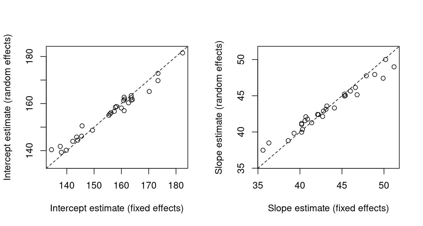
Figure 2.4: Parameter estimates from the random effects model against those from the fixed effects model for the rat growth data
2.4.6 Bayesian inference: the Gibbs sampler
Bayesian inference for LMMs (and their generalised linear model counterparts) generally proceeds using Markov Chain Monte Carlo (MCMC) methods, in particular approaches based on the Gibbs sampler. Such methods have proved very effective.
MCMC computation provides posterior summaries, by generating a dependent sample from the posterior distribution of interest. Then, any posterior expectation can be estimated by the corresponding Monte Carlo sample mean, densities can be estimated from samples etc.
MCMC will be covered in detail in APTS: Computer Intensive Statistics. Here we simply describe the (most basic) Gibbs sampler.
To generate from \(f(y_1,\ldots ,y_n)\), (where the component \(y_i\)s are allowed to be multivariate) the Gibbs sampler starts from an arbitrary value of \(y\) and updates components (sequentially or otherwise) by generating from the conditional distributions \(f(y_i\mid y_{\setminus i})\) where \(y_{\setminus i}\) are all the variables other than \(y_i\), set at their currently generated values.
Hence, to apply the Gibbs sampler, we require conditional distributions which are available for sampling.
For the LMM \[\begin{equation*} Y \sim N(\mu,\Sigma),\quad \mu=X\beta+Zb,\quad b\sim N(0,\Sigma_b) \end{equation*}\] with corresponding prior densities \(f(\beta)\), \(f(\Sigma)\), \(f(\Sigma_b)\), we obtain the conditional posterior distributions \[\begin{align*} f(\beta\mid y,\text{rest})&\propto \phi(y-Zb;X\beta,V)f(\beta)\\ f(b\mid y,\text{rest})&\propto \phi(y-X\beta;Zb,V)\phi(b;0,\Sigma_b)\\ f(\Sigma\mid y,\text{rest})&\propto \phi(y-X\beta-Zb;0,V)f(\Sigma)\\ f(\Sigma_b\mid y,\text{rest})&\propto \phi(b;0,\Sigma_b)f(\Sigma_b) \end{align*}\] where \(\phi(y;\mu,\Sigma)\) is a \(N(\mu,\Sigma)\) p.d.f. evaluated at \(y\).
We can exploit conditional conjugacy in the choices of \(f(\beta)\), \(f(\Sigma)\), \(f(\Sigma_b)\) making the conditionals above of known form and hence straightforward to sample from. The conditional independence \((\beta,\Sigma)\indep \Sigma_b \mid b\) is also helpful.