1.2 Criteria for model selection
1.2.1 Likelihood inference under the wrong model
Suppose the (unknown) true model is \(g(y)\), that is, \(Y_1,\ldots, Y_n\sim g\). Suppose we have a candidate model \(f(y;\theta)\), under which we assume \(Y_1,\ldots, Y_n\sim f(y;\theta)\), which we wish to compare against other candidate models. For each candidate model, we will first find maximum likelihood estimate \(\hat \theta\) of the model parameters, then use some criteria based on the fitted loglikelihood \(\hat \ell = \ell(\hat \theta)\) to compare candidate models.
We do not assume that our candidate models are correct: there may be no value of \(\theta\) such that \(f(.;\theta) = g(.)\). Before we can decide on an appropriate criterion for choosing between models, we first need to understand the asymptotic behaviour of \(\hat \theta\) and \(\ell(\hat \theta)\) without the usual assumption that the model is correctly specified.
The log likelihood \(\ell(\theta)\) will be maximised at \(\hat\theta\), and \[\bar \ell(\hat\theta)=n^{-1}\ell(\hat\theta)\to \int \log f(y;\theta_g) g(y)\, dy,\quad \text{almost surely as } n\to\infty,\] where \(\theta_g\) minimises the Kullback–Leibler divergence \[KL(f_\theta,g) = \int \log\left\{ \frac{g(y)}{f(y;\theta)}\right\} g(y) \, dy.\]
Theorem 1.1 Suppose the true model is \(g\), that is, \(Y_1,\ldots, Y_n\sim g\), but we assume that \(Y_1,\ldots, Y_n\sim f(y;\theta)\). Then under mild regularity conditions, the maximum likelihood estimator \(\hat\theta\) has asymptotic distribution \[\begin{equation} \hat\theta\ \sim\ N_p\left\{ \theta_g, I(\theta_g)^{-1}K(\theta_g)I(\theta_g)^{-1}\right\}, \tag{1.1} \end{equation}\] where \[\begin{align*} K(\theta) &= n \int \frac{\partial \log f(y;\theta)}{\partial\theta} \frac{\partial \log f(y;\theta)}{\partial\theta^T}g(y)\, dy,\\ I(\theta) &= -n \int \frac{\partial^2 \log f(y;\theta)}{\partial\theta\partial\theta^T} g(y)\, dy. \end{align*}\] The likelihood ratio statistic has asymptotic distribution \[W(\theta_g)=2\left\{\ell(\hat\theta)-\ell(\theta_g)\right\}\sim \sum_{r=1}^p \lambda_r V_r,\] where \(V_1,\ldots, V_p\sim \chi^2_1\), and the \(\lambda_r\) are eigenvalues of \(K(\theta_g)^{1/2}I(\theta_g)^{-1} K(\theta_g)^{1/2}\). Thus \(E\{W(\theta_g)\}=\tr\{I(\theta_g)^{-1}K(\theta_g)\}\).
Under the correct model, \(\theta_g\) is the ‘true’ value of \(\theta\), \(K(\theta)=I(\theta)\), \(\lambda_1=\cdots=\lambda_p=1\), and we recover the usual results.
In practice \(g(y)\) is of course unknown, and then \(K(\theta_g)\) and \(I(\theta_g)\) may be estimated by \[\hat K = \sum_{j=1}^n \frac{\partial \log f(y_j;\hat\theta)}{\partial\theta} \frac{\partial \log f(y_j;\hat\theta)}{\partial\theta^T},\quad \hat J = - \sum_{j=1}^n \frac{\partial^2 \log f(y_j;\hat\theta)} {\partial\theta\partial\theta^T};\] the latter is just the observed information matrix. We may then construct confidence intervals for \(\theta_g\) using (1.1) with variance matrix \(\hat J^{-1}\hat K\hat J^{-1}\).
1.2.2 Information criteria
Using the fitted likelihood \(\bar \ell(\hat \theta)\) to choose between models leads to overfitting, because we use the data twice: first to estimate \(\theta\), then again to evaluate the model fit. If we had another independent sample \(Y_1^+,\ldots,Y_n^+\sim g\) and computed \[\bar\ell^+(\hat\theta) = n^{-1}\sum_{j=1}^n \log f(Y^+_j;\hat\theta),\] then we would not have this problem, suggesting that we choose the candidate model that maximises \[\Delta = E_g\left[ E^+_g\left\{ \bar\ell^+(\hat\theta) \right\} \right],\] where the inner expectation is over the distribution of the \(Y_j^+\), and the outer expectation is over the distribution of \(\hat\theta\).
Since \(g(.)\) is unknown, we cannot compute \(\Delta\) directly. We will show that \(\bar \ell(\hat \theta)\) is a biased estimator of \(\Delta\), but by adding an appropriate penalty term we can obtain an approximately unbiased estimator of \(\Delta\), which we can use for model comparison.
We write \[\begin{equation*} E_g\{\bar \ell(\hat \theta)\} = \underbrace{E_g\{\bar \ell(\hat \theta) - \bar \ell(\theta_g)\}}_{a} + \underbrace{E_g\{\bar \ell(\theta_g)\} - \Delta}_{b} + \Delta \end{equation*}\] We will find expressions for \(a\) and \(b\), which will give us the bias in using \(\bar \ell(\hat \theta)\) to estimate \(\Delta\), and allow us to correct for this bias.
We have \[a = E_g\{\bar\ell(\hat\theta) - \bar\ell(\theta_g)\} = \frac{1}{2n}E_g\{W(\theta_g)\} \approx \frac{1}{2n}\tr\{I(\theta_g)^{-1} K(\theta_g)\}.\]
Results on inference under the wrong model may be used to show that \[b = E_g\{\bar \ell(\theta_g)\} - \Delta \approx \frac{1}{2n} \tr\{I(\theta_g)^{-1} K(\theta_g)\}.\] We will not prove this here.
Putting this together, we have \[E_g\{\bar \ell(\hat \theta)\} = \Delta + a + b = \Delta + \frac{1}{n} \tr\{I(\theta_g)^{-1} K(\theta_g)\},\] so remove the bias in using \(\bar\ell(\hat\theta)\) to estimate \(\Delta\), we aim to maximise \[\bar\ell(\hat\theta) - \frac{1}{n}\tr(\hat J^{-1} \hat K).\] Equaivalently, we can maximise \[\hat \ell - \tr(\hat J^{-1} \hat K),\] or equivalently minimise \[2\{\tr(\hat J^{-1}\hat K)-\hat\ell\},\] the Network Information Criterion (NIC).
Let \(p=\dim(\theta)\) be the number of parameters for a model, and \(\hat\ell\) the corresponding maximised log likelihood. There are many other information criteria with a variety of penalty terms:
- \(2(p-\hat\ell)\) (AIC—Akaike Information Criterion)
- \(2(\frac{1}{2} p\log n-\hat\ell)\) (BIC—Bayes Information Criterion)
- AIC\(_\text{c}\), AIC\(_\text{u}\), DIC, EIC, FIC, GIC, SIC, TIC, \(\ldots\)
- Mallows \(C_p=RSS/s^2 + 2p-n\) commonly used in regression problems, where \(RSS\) is residual sum of squares for candidate model, and \(s^2\) is an estimate of the error variance \(\sigma^2\).
Example 1.2
AIC and BIC can both be used to choose between the \(2^5\) models previously fitted to the nodal involvement data. In this case, both prefer the same model, which includes three of the five covariates:acid, stage and xray (so has four free parameters).
Figure 1.2 shows the AIC and BIC for each model, against the number of free parameters. BIC increases more rapidly than AIC after the minimum, as it penalises more strongly against complex models.
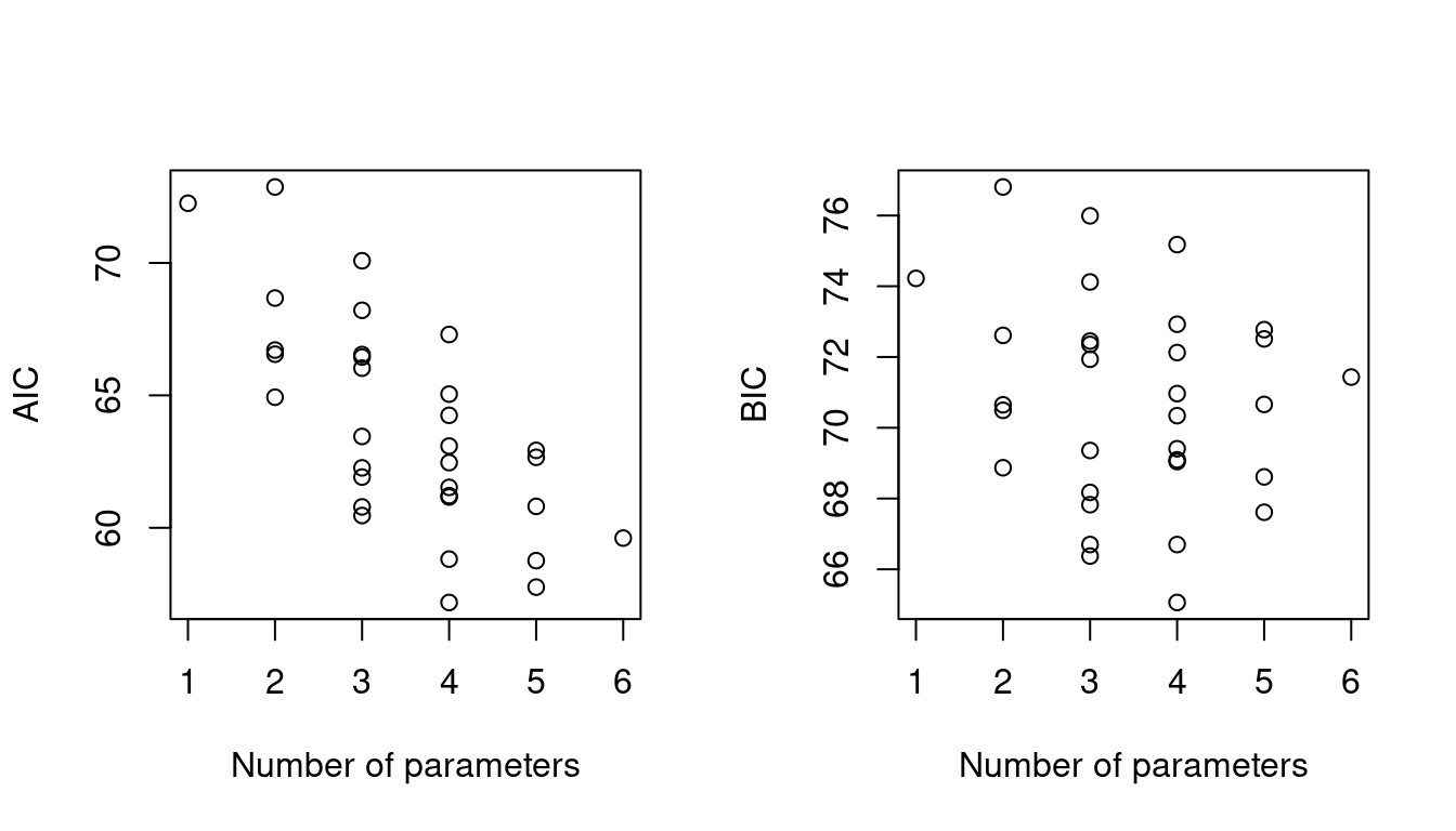
Figure 1.2: AIC and BIC for 32 possible logistic regression models for the nodal data
1.2.3 Theoretical properties of information criteria
We may suppose that the true underlying model is of infinite dimension, and that by choosing among our candidate models we hope to get as close as possible to this ideal model, using the data available. If so, we need some measure of distance between a candidate and the true model, and we aim to minimise this distance. A model selection procedure that selects the candidate closest to the truth for large \(n\) is called asymptotically efficient.
An alternative is to suppose that the true model is among the candidate models. If so, then a model selection procedure that selects the true model with probability tending to one as \(n\to\infty\) is called consistent.
We seek to find the correct model by minimising \(\text{IC}=c(n,p)-2\hat\ell\), where the penalty \(c(n,p)\) depends on sample size \(n\) and model dimension \(p\)
- Crucial aspect is behaviour of differences of IC.
- We obtain IC for the true model, and IC\(_+\) for a model with one more parameter.
Then \[\begin{align*} P(\text{IC}_+<\text{IC}) &= P\left\{ c(n,p+1)-2\hat\ell_+< c(n,p)-2\hat\ell\right\}\\ &= P\left\{2(\hat\ell_+-\hat\ell) >c(n,p+1)-c(n,p)\right\}. \end{align*}\] and in large samples \[\begin{align*} \mbox{ for AIC, } c(n,p+1)-c(n,p) &= 2\\ \mbox{ for NIC, } c(n,p+1)-c(n,p) &\approx 2\\ \mbox{ for BIC, } c(n,p+1)-c(n,p) &= \log n \end{align*}\]
In a regular case \(2(\hat\ell_+-\hat\ell)\sim\chi^2_1\), so as \(n\to\infty\), \[ P(\text{IC}_+<\text{IC}) \to \begin{cases} 0.16,&\text{AIC, NIC},\\ 0,&\text{BIC}. \end{cases} \] Thus AIC and NIC have non-zero probability of over-fitting, even in very large samples, but BIC does not.