1.3 Variable selection for linear models
Consider a normal linear model \[Y_{n\times 1} = X^\dagger_{n\times q}\beta_{q\times 1} + \epsilon_{n\times 1},\quad \epsilon \sim N_n(0,\sigma^2I_n),\] with design matrix \(X^\dagger\) with columns \(x_r\), for \(r\in\mathcal{X}=\{1,\ldots, q\}\). We choose a model corresponding to a subset \(\mathcal{S} \subseteq \mathcal{X}\) of columns of \(X^\dagger\), of dimension \(p = |S|\).
Terminology:
- the true model corresponds to the subset \(\mathcal{T}=\{r:\beta_r\neq 0\}\), and \(|\mathcal{T}|=p_0<q\);
- a correct model contains \(\mathcal{T}\) but has other columns also, corresponding subset \(\mathcal{S}\) satisfies \(\mathcal{T}\subset\mathcal{S}\subset\mathcal{X}\) and \(\mathcal{T}\neq\mathcal{S}\);
- a wrong model has subset \(\mathcal{S}\) lacking some \(x_r\) for which \(\beta_r\neq 0\), and so \(\mathcal{T}\not\subset\mathcal{S}\).
We aim to identify \(\mathcal{T}\). If we choose a wrong model, we will have bias, whereas if we choose a correct model, we may increase the variance. We seek to choose a model which balances the bias and variance.
To identify \(\mathcal{T}\), we fit a candidate model \(Y=X\beta+\epsilon,\) where columns of \(X\) are a subset \(\mathcal{S}\) of those of \(X^\dagger\). The fitted values are \[X\hat\beta=X \{ (X^T X)^{-1}X^T Y\} =HY = H(\mu+\epsilon) = H\mu + H \epsilon,\] where \(H=X(X^T X)^{-1}X^T\) is the hat matrix and \(H\mu=\mu\) if the model is correct
Following the reasoning for AIC, suppose we also have independent dataset \(Y_+\) from the true model, so \(Y_+=\mu+\epsilon_+\). Apart from constants, previous measure of prediction error is \[\Delta(X)=n^{-1}E E_+\left\{(Y_+-X\hat\beta)^T(Y_+-X\hat\beta)\right\},\] with expectations over both \(Y_+\) and \(Y\).
Theorem 1.2 We have \[\begin{align*} \Delta(X) &= n^{-1}\mu^T(I-H)\mu + (1+p/n)\sigma^2 \\ &= \begin{cases} n^{-1}\mu^T(I-H)\mu + (1+p/n)\sigma^2 & \text{if model is wrong,}\\ (1+p_0/n)\sigma^2 & \text{if model is true,}\\ (1+p/n)\sigma^2 & \text{if model is correct.} \end{cases} \end{align*}\]
The bias term \(n^{-1}\mu^T (I-H)\mu>0\) unless the model is correct, and is reduced by including useful terms. The variance term \((1+p/n)\sigma^2\) is increased by including useless terms. Ideally we would choose covariates \(X\) to minimise \(\Delta(X)\), but this is impossible, as it depends on unknowns \(\mu,\sigma\). We will have to estimate \(\Delta(X)\).
Proof. Consider data \(y=\mu+\epsilon\) to which we fit the linear model \(y=X\beta+\epsilon\), obtaining fitted values \[X\hat\beta = Hy = H(\mu+\epsilon) \] where the second term is zero if \(\mu\) lies in the space spanned by the columns of \(X\), and otherwise is not.
We have a new data set \(y_+=\mu+\epsilon_+\), and we will compute the average error in predicting \(y_+\) using \(X\hat\beta\), which is \[\Delta=n^{-1}E\left\{(y_+-X\hat\beta)^T(y_+-X\hat\beta)\right\}.\] Now \[y_+-X\hat\beta = \mu+\epsilon_+ - (H\mu + H\epsilon) = (I-H)\mu + \epsilon_+ - H\epsilon.\] Therefore \[(y_+-X\hat\beta)^T(y_+-X\hat\beta) = \mu^T (I-H)\mu + \epsilon^T H\epsilon + \epsilon_+^T\epsilon_+ + A\] where \(E(A)=0\), which gives the result.
Example 1.3
We consider an example with \(n=20\), \(p_0=6\), and \(\sigma^2=1\). In this example, the true model is a a degree five polynomial. Figure 1.3 shows \(\log(\Delta(X))\) for models of increasing polynomial degree, from a quadratic model (\(p = 3\)) to a degree 14 polynomial (\(p = 15\)).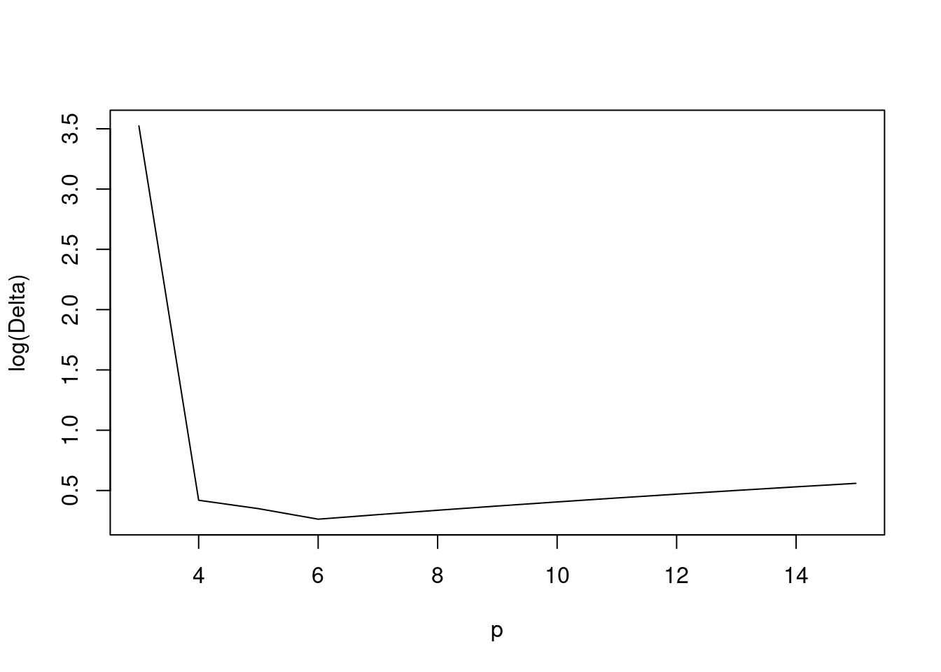
Figure 1.3: \(\log(\Delta(X))\) for models with varying polynomial degree
The minimum of \(\Delta(X)\) is at \(p=p_0=6\): There is a sharp decrease in bias as useful covariates are added, and a slow increase with variance as the number of variables \(p\) increases.
If \(n\) is large, can split the data into two parts \((X',y')\) and \((X^*,y^*)\), say, and use one part to estimate the model, and the other to compute the prediction error; then choose the model that minimises \[\hat\Delta = \frac{1}{n'}(y'-X'\hat\beta^*)^T(y'-X'\hat\beta^*) = \frac{1}{n'}\sum_{j=1}^{n'}(y_j'-x_j'\hat\beta^*)^2.\] Usually the dataset is too small for this, so we often use leave-one-out cross-validation, which is the sum of squares \[ n\hat\Delta_\text{CV} = \text{CV}=\sum_{j=1}^n (y_j-x_j^T\hat\beta_{-j})^2,\] where \(\hat\beta_{-j}\) is estimate computed without \((x_j,y_j)\). This seems to require \(n\) fits of model, but in fact \[\text{CV} =\sum_{j=1}^n \frac{(y_j-x_j^T\hat\beta)^2}{(1-h_{jj})^2},\] where \(h_{11},\ldots, h_{nn}\) are diagonal elements of \(H\), and so can be obtained from one fit.
A simpler (and often more stable) version uses generalised cross-validation, which is the sum of squares \[\text{GCV} =\sum_{j=1}^n \frac{(y_j-x_j^T\hat\beta)^2}{\{1-\tr(H)/n\}^2}.\]
Theorem 1.3 We have \[E(\text{GCV}) = {\mu^T(I-H)\mu/(1-p/n)^2} + n\sigma^2/(1-p/n)\approx n\Delta(X).\]
Proof. We need the expectation of \((y-X\hat\beta)^T(y-X\hat\beta),\) where \(y-X\hat\beta = (I-H)y = (I-H)(\mu+\epsilon),\) and squaring up and noting that \(E(\epsilon)=0\) gives \[E\left\{ (y-X\hat\beta)^T(y-X\hat\beta)\right\} = \mu^T(I-H)\mu + E\left\{\epsilon^T(I-H)\epsilon\right\} = \mu^T(I-H)\mu +(n-p)\sigma^2.\] Now note that \(\tr(H)=p\) and divide by \((1-p/n)^2\) to give (almost) the required result, for which we need also \((1-p/n)^{-1} \approx 1+p/n\), for \(p\ll n\).
We can minimise either \(\text{GCV}\) or \(\text{CV}\). Many variants of cross-validation exist. Typically we find that model chosen based on CV is somewhat unstable, and that GCV or \(k\)-fold cross-validation works better. A standard strategy is to split data into 10 roughly equal parts, predict for each part based on the other nine-tenths of the data, then find the model that minimises this estimate of prediction error.